


Fault Tree Analysis (FTA) is a deductive and structured method to determine the root causes and fault combinations of a system failure using a graphical model. In addition, quantification of a fault tree allows the assessment of the probability of system unavailability and unreliability to compute the quantitative target values of a safety standard. For example, IEC61508 defines the Probability of Failure on Demand (PFD) for low-demand systems and the Probability of Failure per Hour (PFH) for high-demand or continuous-demand systems, ISO 26262 the PMHF metric, and so on.
The medini analyze FTA module supports "stand alone" modeling of fault trees as well as a connected analysis based on a system design model or other analysis data. Thereby, the fault tree is semi-automatically created from a model and quantitative parameters are derived, for example, from FIT rates of components, failure nets, or safety mechanisms of an FME(D)A. Moreover, the fault tree is synchronized whenever the underlying design model changes. This allows an accurate and always up-to-date fault tree analysis.
In addition to classic fault trees, the tool supports Component Fault Trees (CFT). This allows for a more advanced model-based approach by bringing fault trees and SysML design even closer together. For more details, see Component Fault Trees (CFT).
Note that the FTA-related features for quantitative analysis are only available if there is a valid Premium or Enterprise license installed. For licensing details, see License Configuration.
All FTA models are managed in FTA packages of a project. The location depends on the safety domain profile and project template, see Safety Domain Profiles for more details.
In order to create a new fault tree do the following:
Choose "New -> FTA Model ..." from the context menu of a FTA package (or any sub-package thereof).
Provide a name for the FTA model and the top-level event
After pressing OK the new FTA model will be created and an initial diagram is opened that is empty with the exception of the top-level event.
In addition certain project templates support the creation is also available on selected element, depending on the safety domain. For example, in ISO 26262, as a short-cut, "Derive -> FTA Model..." may be invoked from the context menu of a safety goal. In these cases the target package for the FTA model has to be specified additionally in the upcoming dialog.
Note that newly created FTA models are in this case also traced, i.e. a trace between the safety goal and the FTA model is created while creating the new FTA model.
The FTA editor is opened automatically after creating a new FTA model, by double-clicking on the diagram icon of the FTA model in the Model Browser, or by choosing "Open Diagram" from the context menu of that entry.
As all graphical editors, the FTA editor features a palette that can be used to create events and gates as well as a property view to edit their detailed properties. In addition, an outline view is supported that provides a quick access to elements in the fault tree or a graphical outline (see Outline view).
Each event node contains the following information:
Event name/description in the top compartment (rectangular text box).
Event identifier in the middle compartment that is initially assigned automatically based on an auto-numbering (see Auto-counter Patterns). The shape of this middle "decoration" compartment indicates the type of the event (see further below).
Event probability and failure frequency labels (optional). These labels are shown below the middle compartment for primary events and within the middle compartment for intermediate and top level events.
All values can be modified directly in the diagram (text and ID) or in the properties view (see Event and Gate Properties ) for the selected event or gate.
Different event types are supported. The event type is indicated by different shapes for the middle compartment (i.e. the "event type decoration"):
TOP_LEVEL: top level events are indicated by a rectangle. All events are marked automatically as top-level if they have an incoming connection (i.e. gate or intermediate event) and if they're not referenced via a transfer gate. Hence, the kind cannot be set manually to TOP_LEVEL.
INTERMEDIATE: an event that occurs because there are one or more causing events to the intermediate event usually connected via a logical or transfer gate. Note that events are automatically changed to intermediate events, once the event is connected to other nodes so that it is in between these nodes. Therefore, the kind cannot be set manually to INTERMEDIATE.
BASE: basic events that define a not further refined failure or condition; usually used as leave elements in the fault tree. This is the default type for new events.
HOUSE: background condition, usually can be taken for granted. The value of this event has often a probability of 1.0 to just document some condition to be present or 0.0, if the condition is never met. During fault tree evaluation, these events will be treated like a BASE event.
UNDEVELOPED: basic event that has not been further analyzed and though it is supposed to consist of other base/intermediate events that trigger this event, although these sub-events are not detailed in the current fault tree. During fault tree evaluation, these events will be treated like a BASE event.
CONDITIONAL: an event used to specify conditions for the occurrence of a failure or a condition of the system or a component. During fault tree evaluation, these events will be treated like a BASE event.
In general there are three ways to add new events to a fault tree:
Directly creating new events onto the diagram using the "Event" entry from the editor's palette. You can drop a new event onto an existing gate, base event or onto a connection to insert it between existing nodes. After creation, you have to specify at least the name for the newly created event; an identifier will be inserted automatically.
Deriving new events from other model elements. This allows to automatically derive parts of the fault tree and synchronize e.g. reliability data with other analyses such as FME(D)A. See Creation of Events from Models) for further details.
Creating new events from the outline view. Dragging basic events from the FTA outline view allows you to insert quickly a multiple occurring event (MOE) or a transfer gate to an existing branch that is already referenced, i.e. a multiple occurring branch (MOB). See Reoccurring Eventsas well as Outline view for details.
Using the different gate types from the drawing palette you can develop the tree logic by introducing gates and connections between events as required. The following gate types are available in the FTA editor:
AND-Gate, OR-Gate, XOR, and NOT-Gates: these correspond to the usual logical operators
Please note you can change the type of an existing gate using the properties view for the gate and selecting the type from the drop-down list
Voting-Gate: Corresponds to an n-out-of-m selection where n is the threshold property of the voting gate and m the number of operands for that gate. The threshold property can be changed using the property view.
Transfer-Gate: Allows to continue the tree at an already existing event or fault tree. The target event (i.e. where the tree shall be continued) must be selected from a dialog which opens automatically when a transfer gate is created. For details see Reoccurring Events.
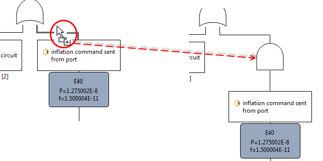
Gates and events can be moved by drag & drop from the palette directly onto existing events or gates in a diagram. This will automatically connect the event/gate to the node on which it has been dropped. Moreover, it is possible to change (refactor) already connected elements in the tree through node insertion. Dropping an event/gate on an existing connection (line) will insert the event/gate at that position in the tree and reconnect the upper/lower nodes accordingly (here for an AND gate from the palette):
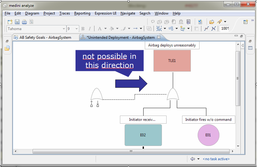
In certain situations it might be required to place the gate symbol on any free place in the diagram, e.g. for refactoring tasks. In these cases the connection from the event to the gate has to be drawn explicitly with the "Connect" element from the palette. Please note that the tool observes the direction of the line creation and it will forbid wrong connections as well as cycles. The connection line is working in "top-down" direction, i.e. start of the connection is always the position in the tree where the target element shall be connected to as input.
Events can also by freely created on any diagram. These events are then by default not connected and appear in the model browser directly under the fault tree model. The connection to the fault tree must be established in the same way by using the connection line.
Fault trees can be shown on multiple diagrams and all FTA diagrams can show any part of a fault tree. Some tools bind diagramming to transfer gates, which is not the case in Ansys medini analyze. It makes sense to setup some ground rules for diagram partinioning before starting the analysis, e.g. make use of transfer gates or restrict the gate levels shown on a diagram.
Note that there are two ways to create or paginate diagrams:
Create a new empty diagram or child diagram in the Model Browser by simply selecting "New | Diagram" on an FTA model or "Create Child diagram" on a diagram.
Afterwards, you can drag and drop existing events onto the diagram and e.g. use "Restore subtree" to create visual representations of the events.
Create a diagram by revising/splitting an existing diagram. You can do this by selecting an event on a diagram and choose "Move to Child Diagram" from the context menu. This will create a new diagram and initialize it with the complete subtree from below the selected event.
This feature allows you to optionally insert a transfer gate so that you can break up the tree structure with a transfer if desired. If no transfer is used, a small triangle similar to a transfer will indicate that the tree is continued elsewhere (see also Laying Out a Fault Tree).
Reoccurring parts are common in almost any fault tree analysis. The tool supports two ways to reference an existing event or subtree:
Transfer gates: Transfer gates are essentially the referencing mechanism in fault tree analysis. They allow to point to a so called target event at which the fault tree (logic) is further refined. Thereby transfer gates can be used in three ways:
Continue a fault tree on a new diagram (pagination). Thereby the target event is referenced in the first place only from one place, i.e. the transfer gate. This is the case in most FTA tools, see also FTA Diagram Pagination.
Reference an intermediate event as subtree, which creates a multiple occurring branch (MOB). This effectively creates a graph out of the fault tree.
Continue a fault tree at an (intermediate or basic) event of another fault tree. In this way reuse of (part of) another FTA can be hooked into the current fault tree.
The details and implications of these three usages are explained further below in this section.
Multiple Occurring Events (MOE): Primary events that occur multiple times can be added to the fault tree using a special MOE event. Thereby, the same event is added to multiple places in the current fault tree. Note that MOEs are limited to the scope of a single FTA model. They can be created easily from the outline view (cp.Outline view).
We'll discuss the details of transfer gates and MOEs that are required to understand how these relate to each other in the following. Creating a transfer gate from the palette will open a normal selection dialog:
Note that the target event selection prohibits the creation of loops in a fault tree. Therefore, events that would lead to loop in the fault tree are not shown in the selection.
If the button "Create without target" is selected, the target is not set and can be set (or changed) later by invoking the "Show properties view" from the context menu of the transfer gate on the diagram.
Transfer gates into other fault trees of the same project are supported and shown in the selection dialog. In this case, the transfer gate symbol will be decorated with a small arrow in the bottom right corner as shown below:
Double click on a transfer gate navigates to the target event by opening the diagram and selecting the event.
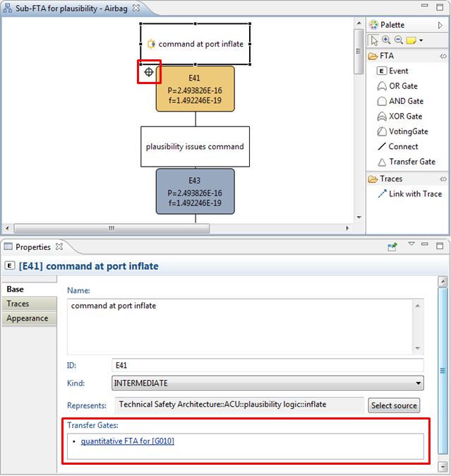
On the opposite side, the event referenced by one (or more) transfer gates receives a decoration as shown in the screenshot below. Navigation back to the transfer gate(s) can be achieved via the property view link (opening the corresponding diagram) or via the context menu "Related Elements -> Transfer Gates". Note that the related elements will navigate into the model browser.
Please note it is generally not required for the target event to be shown on the same diagram or on any diagram at all. Therefore, transfer gates provide a general mechanism to reference any event in the same project (with the exception that loops are not allowed). During evaluation, the transfer gates are followed to determine the full scope of analysis (cp. Analysis of Fault Trees).
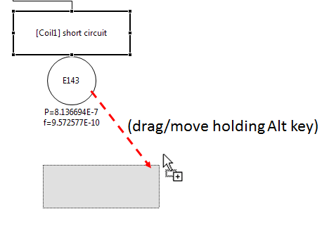
If only a basic event shall be inserted at multiple places in a fault tree, a MOE can be created instead of a transfer gate. A MOE can be easily created by move (drag) pressing the Alt key on a diagram like this:
An alternative to create MOEs is to use the Outline View for FTA, see Outline view.
The layout of a fault tree is automated to a large extent. Inserting events and gates will automatically lead to an auto-arranged tree. In addition, a manual refinement is always possible at any time later. This allows to create an optimal graphical layout with minimum manual effort.
There are two main adjustments that influence the default layout and positioning of elements:
Workspace preferences for FTA: new diagrams are initialized with the default settings given under "Window | Preferences -> Diagrams | FTA". Especially the general spacing for the auto-layout is set on the "Diagram | FTA | Layout" page.
Project settings for FTA: each project itself defines how events are layouted by default. The options are:
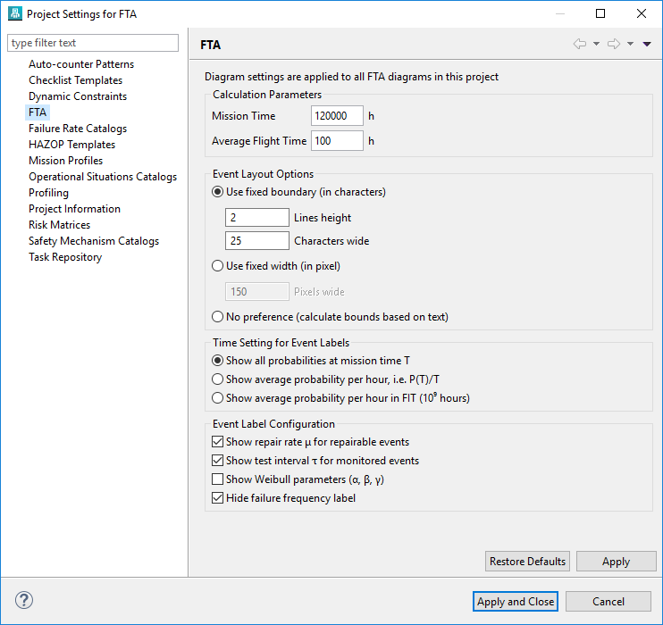
The option "Use fixed boundary (in characters)" sets the text area to a size so that n text lines with m characters each fit into the rectangle. Alternatively, the event can be set to a fixed width with option "Use fixed width (in pixel)", leading to line-breaks and vertical extension of the rectangle when the text exceeds one line. If the last option "No preference" is chosen, no line breaks of text will be applied and you are responsible to resize the event as required.
Note that in all cases the event size can be set manually after events have been created. So for example if option "Use fixed boundary" is used and a text doesn't fit into the area, a manual resize is possible.
In addition, the following functions can be used to improve and/or tailor the layout as required:
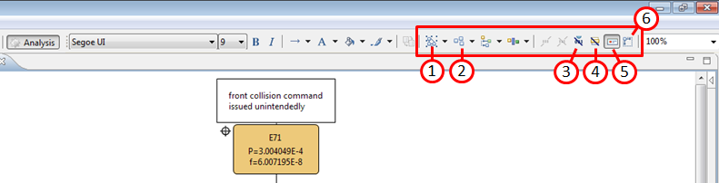
The quick selection of all elements in the diagram is supported by the "Select All", "Select All Shapes", and "Select All Connectors" button. It can be used in combination with the re-arrange button (2) or with the resize button (6), e.g. if the default spacing or event text options have been changed.
The nodes of a fault-tree on the diagram (or just the selected elements) can be automatically re-arranged using the "Arrange All" and "Arrange Selected" button. Note that also the context menu entry "Arrange Subtree" on a fault tree node can be used alternatively without selecting the subtree explicitly.
This button switches the display of the probability labels of events on and off. If purely qualitative fault trees are developed, this function can hide unnecessary probability and failure frequency labels.
Option to hide the intermediate event IDs. If you use gate labels to identify subtrees in a fault tree, you might find it useful to hide the identifiers in order to have no duplicate or irritating numbering. In combination with (3), intermediate events are reduced to pure text boxes to save space.
Toggle button for icons of events. All events that have a represents reference can show the icon of the element next to the text of the event like this:
The "Auto Size" button (re-)sets the element width and height to the default, i.e. the settings in the FTA project. This is useful e.g. if the event size options have been changed (see above). In this case all events can be quickly re-layouted by selecting all elements on the diagram and then selecting the "Auto Size" button.
In order to easily handle also large fault trees medini analyze provides a few additional functions for the FTA editor:
Usage of multiple diagrams: You can add additional diagrams to a FTA model using the context menu of the model in the Model Browser. This allows to specify the full fault tree as a set of sub-trees (each on it's own diagram). The connections to construct the complete tree from the single sub-trees are defined using transfer gates. See Reoccurring Events for details.
Tree-Folding: By double-clicking on a tree element (event or gate) the sub-tree starting at that element can be folded (i.e. temporarily hidden from the diagram) - the element will in this case be decorated with a folding indicator (small plus symbol in the upper right corner, see below). Double-clicking on an element with a folding indicator will restore the sub-tree starting at that element again.
Note if a folded node has been moved to a different place on the diagram, the unfolding will also start from this new location. The animation of (un-)folding of trees can be influenced in the preferences menu (Window | Preferences -> Diagrams | FTA | Subtrees).
If incoming nodes of a fault tree are hidden from a diagram, either because they are deleted from the diagram or because they are folded in, a hidden elements indication is shown at the nodes (small triangle, see 1):
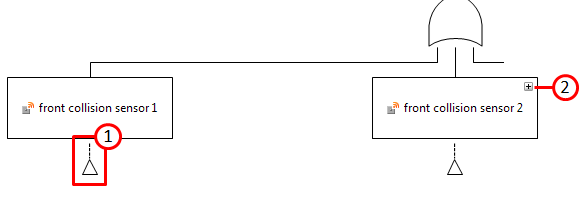
The small triangle indicates that there is a subtree (or at least one element) below that event and its notation is inspired by the transfer gate, which has the same semantics. The indication will also be present if a subtree is folded in (see 2). In the latter case, double clicking will restore the tree. In the former case the subtree elements can be selectively dragged (back) onto the diagram from the Model Browser. As an alternative, subtrees can be restored using the context menu entry Restore subtree. This will recreate all graphical views of the whole subtree until all leaf nodes are reached.
In order to edit detailed information of the elements in a fault tree, the property view is used. The property view shows all informations of the selected element. You can select the element either on the diagram or in the model browser.
Please note if the properties view is not shown, you can open it by choosing Show Properties View from the context menu of an event in the editor or the model browser.
Depending on the type of the selection (gate, event, diagram, model), the property view shows different tabs. The Trace Tab, Appearance Tab, and Rulers & Grid Tab are generic tabs. See the appropriate sections for details. In case profile properties have been defined for fault tree elements (see Profiling mechanism) you can assign values in the tab Profile of the property view. You will see the list of all user defined properties for the selected element (if a profile is defined).
Specific tabs exist for events, gates and the diagram/model. Note that clicking an empty space in the diagram shows the properties for the whole FTA model (similar to selecting the FTA model node in the model browser.)
In the Base tab of Events the following properties can be set:
Name: The name of the event
Kind: The kind of the event - BASE, HOUSE, UNDEVELOPED, CONDITIONAL. Event kind INTERMEDIATE and TOP_LEVEL will be automatically determined if the event is connected to other nodes of the tree.
Id: The ID of the event
Represents: the element that the event represents (so called derived events). Properties of the referenced element can be used to derive the probability of the event.
Transfer Gates: Links to the transfer gates connected with (targeting) the actual element. This field is not editable. The links can be clicked to navigate to the transfer gate.
On the Probability tab, the probability model can be configured. Currently, medini analyze supports the following kind of probability models:
Fixed probability. Constant value between [0..1] that is not changing over time.
Time independent derived probability. Basically the same as the fixed model, but the value is derived from the represented model element:
For safety mechanisms, the probability can be derived from the diagnostic coverage values. There are four options:
Diagnostic Coverage of single point faults: p = DCSPF
Residual fault fraction: p = 1 - DCSPF
Diagnostic Coverage of latent faults: p = DCLF
Latent fault fraction: p = 1 - DCLF
For all other elements the probability will be p = 0.
Exponential distribution. The probability P(E) of an event E based on the exponential distribution with constant failure rate is given by the formula:
P(E) = 1- e-λt
where λ is the event's failure rate (in hours) and t the mission time (in hours).
Exponential distribution with constant repair rate (i.e. "repairable events"). If failures of components can be repaired within a constant repair time, the probability P(E) is defined by the following formula (if the component is considered to be as good as new after repair):
P(E) = λ/(λ+μ) * (1- e-(λ + μ)t)
where λ is the failure rate of the component (in hours), μ the repair rate (per hour), and t the mission time (in hours). Note that the repair rate can be determined from the Mean Time To Repair (MTTR) using the formula: μ = 1/MTTR.
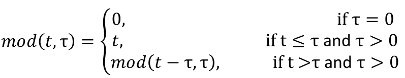
Exponential distribution with test/monitoring interval (i.e. "monitored events"). If components are monitored periodically and failures lead to a replace/repair of the component, the probability of failure p(E) of an event is determined by the formula:
P(E) = 1- e-λmod (t, tau)
where λ is the failure rate of the component (in hours), tau the test interval (in hours), t the mission time (in hours), and mod a specialized modulo function that is defined as follows:
Risk Time Model: specific probability model as typically used in Aerospace contexts. The computational semantics for time dependent evaluations is the same as the exponential distribution with a monitoring interval:
P(E) = 1- e-λmod(t, T_r)
The risk time T_r (maximum time at risk) can be set to either the mission time, average flight time, or any specific time. The difference compared to a monitored event is only when computing Q_avg and Q_wc (see Evaluation Results of a Fault Tree).
Weibull distribution. The probability of an event P(E) with Weibull failure distribution is given by the formula:
P(E) = 1- e-( max{t - g, 0} / a )beta
where beta is the shape parameter, a the scale parameter, g the time shift (in hours), and t the mission time (in hours).
Selecting True/False allows an event to be always TRUE (verum) or FALSE (falsum). This model gives an event actually not a probability, but the event will be evaluated always as either true or false in the boolean context of the fault tree. Note that the effect on the fault tree depends on how the true/false event is connected and whether it is TRUE or FALSE. For example, a FALSE event connected to an AND gate will eliminate the evaluation of all other branches going into the AND, effectively serving as a "switch".
Custom. A custom probability distribution allows users to provide almost any mathematical expression or script to calculate the probability P(E). Hence, any missing distribution can be added in case it is missing in the list of distributions above.
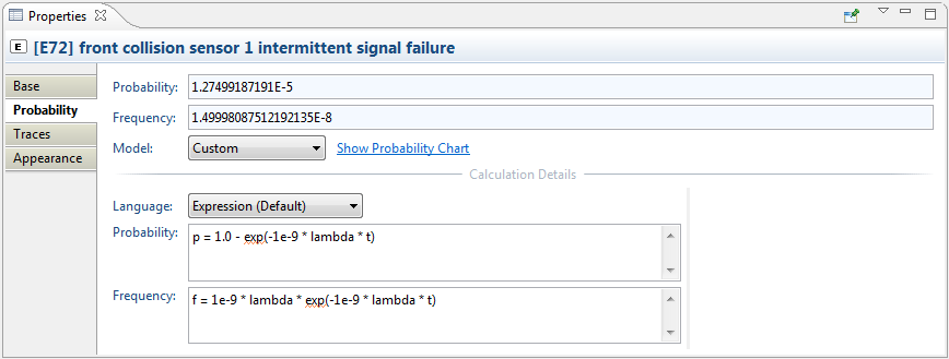
The screenshot below shows the general structure of the Probability tab along the exponential probability distribution:
The top three fields Probability, Frequency, and Model are common and always shown, the lower part of the page is dependent on the the selected probability Model:
Probability: The probability P(E) at mission time T of the FTA model. If the probability is set to Fixed, the value can be directly edited, otherwise it is computed from the settings below. P(E) is shown on the FTA diagram as probability label "P=..." at the event.
Frequency: The probability density function (failure frequency) for P(E) at mission time T of the FTA model (i.e. first derivative of the probability function). If the probability is set to Fixed or Time Independent, the value is 0, for repairable events it corresponds to w(t). The frequency is shown on FTA diagrams as label "f=..." at events in both cases.
Model: The selected probability model (see list above). Depending on the selection the property page will be adapted to the input required for each model.
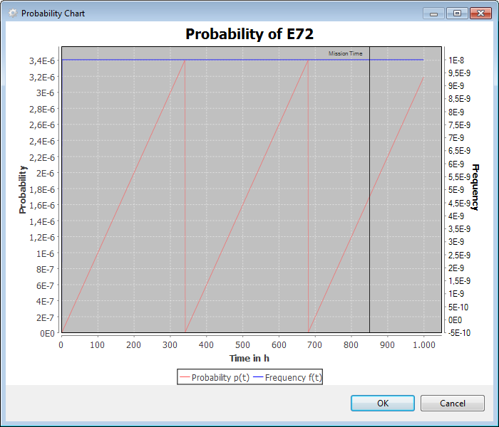
Show Probability Chart: The link next to the probability model opens a chart that visualizes the probability distribution function over time. The plot shows time on the x-axis as well as P(t) and f(t) on the y-axis. Note that these two plots have different scale on the y-axis: scale for the Probability is indicated on the left side while Frequency is indicated on the right side.
In the following subsection the additional fields of the probability tab are explained. Except Fixed, all distributions require additional parameterization.
Exponential distribution:
Failure Rate: Calculation of the probability based on a user specified failure rate (given in FIT)
Use Rate From: Calculation of the probability based on the failure rate of a model element related to the event (i.e. the represented element). In case the event has a represented element set the element's failure rate is used to compute automatically the probability and it will be synchronized (updated) whenever the element changes.
Depending on the type of represented element the probability is computed as follows:
For SysML model elements (parts, ports, blocks) the failure rate is used and P(E) is computed out of the FIT rate λ (converted into hours).
For failure modes contained in models the failure rate of the failure mode is used, i.e. either the fraction of the failure rate according to the distribution or the sum of FIT rates of all causing failure modes.
However, if the default rules for derivation of the probability are not applicable in a specific context, you may also directly specify in the Failure Rate field at the event. The procedure how to create events and link them automatically to design model elements is explained in Creation of Events from Models.
Cycle kind: Refines the exponential distribution and changes it into either a repairable or monitored event (see explanations above). For repairable events the repair rate μ must be specified, for monitored events the test interval τ.
Risk Time Model: (Aviation/Aerospace specific)
The risk time model has the same parameters than the exponential distribution, expect that cycle kind is implicitly set by the "Risk Time Interval". The Risk Time Interval can be selected from three options:
Mission time: The mission time T is used as test interval, i.e. the event is actually not tested. This is the same as a normal exponential distribution.
Average Flight Time: The average flight time is inherited from the project settings for average flight length. This means that the event probability reaches its maximum at the end of a flight and is "reset" for the next flight. For example, this is typically the case for all equipment that is checked before each flight.
Specific time: If an test interval is different from the average flight or mission time, the specific time can be used to model any longer inspection interval. Note that if the given interval is less than an average flight, it means the test happens during flight.
Time Independent distribution:
Use Rate From: Sets the represents reference to the element from which a constant probability shall be derived. Currently, only safety mechanisms are supported for which p = 1 - DC% (related to single point faults).
Weibull:
Alpha: the scale parameter
Beta: the shape parameter
Gamma: initial time shift in hours
Custom (scripted probability):
Language: The scripting language used for defining the probability/failure frequency. Possible values are Expression (default), OCL, and JavaScript (if enabled in preferences). Expressions can be used if a simple mathematical distribution formula shall be assigned to the event (see also Expressions Language). The latter two options, OCL and JavaScript, provide additional access to the full analyze models via navigation and query APIs. See examples below how this can be achieved.
Probability: Expression for the event's probability. If the medini expression language is selected, a mathematical expression must be given and assigned to the predefined variable p. For example, a simple histogram with the probability values 0.2 in [0..100], 0.5 in [100..500], and 0.7 any other time looks like:
p = ifThenElse(less(t, 100), 0.2, ifThenElse(less(t, 500), 0.5, 0.7));
The expression can use the predefined values t for the point of evaluation time (in hours) as well as lambda (in FIT) for the failure rate of the represented element. For more information on the expression language, see Expressions Language. Make sure that the expression evaluates to a probability in the range of [0..1] in all cases, otherwise the behaviour is undefined.
For OCL and JavaScript as language, no variable assignment is required and the last expression is evaluated as probability. In addition to t and lambda, the variable element can be used to access the event element and start accessing model information.
Frequency: The failure frequency is the probability density function. It can be defined in the same way as the probability expression above and it has also access to the same variables.
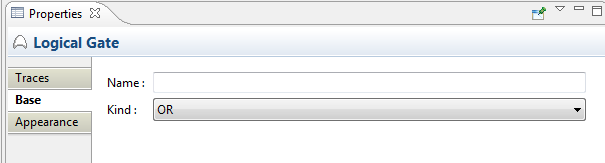
In the Base tab of gates, the following information can be set:
Name: The name of the gate
Kind: In case of logical gates the kind of the logical operation expressed by the gate: AND, OR, XOR, or NOT.
Threshold: In case of a voting gate the threshold above which the gate will fire.
Target Event: The target event in case of a transfer gate to be selected from a selection dialog.
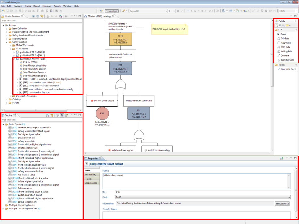
The Outline View for FTA supports the quick lookup of basic and intermediate events that are (potentially) frequently used as well as a graphical bird-eye view on the current diagram. The view can be activated via the menu Window | Show View -> Outline View and looks like follows:
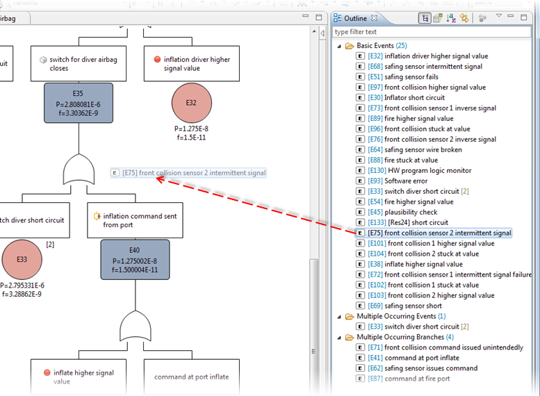
The event outline by default shows three categories of events, each decorated with the number of contained items in parentheses:
Basic Events lists all primary events (leaf events) of the fault tree model
Multiple Occurring Events lists all primary events that occur more than once in the current fault tree model
Multiple Occurring Branches lists all intermediate events that are referenced via transfer gates
The view can be interactively used to further develop the fault tree using drag and drop. If a basic event is dragged from the view onto an event or gate, another occurrence of the event is created. Note that this only works if the event is dropped onto another node: if it is dropped on an empty space in the diagram only the graphical representation is created! If you desire to create anyway a MOE, simply hold down the Alt key while dragging.
Dragging MOEs is also supported to create further occurrences. Similarly, drag and drop of intermediate events from the Multiple Occurring Branches (MOBs) section will create new transfer gates referencing the MOB.
Events of a fault tree can be connected to model elements in SysML models or collections. By referencing an element, the event can inherit properties for the fault tree analysis, e.g. name or failure rate to derive its probability of occurrence. Such events are said to "represent" the failure or element (see also Event and Gate Properties ).
In order to create events from model elements, you have two options:
Drag and drop elements from the Model Browser into an open FTA diagram. It is possible to select and drop multiple elements at once.
Hint: if elements are dropped onto gates or primary events, they are automatically connected on the fly.
In case an element contains failures such as a SysML part, there is an option to insert the element together with its failures. If this option is selected, the element and all of its failures are inserted as events in the fault tree and they are connected under an OR gate.
As alternative, you can select elements of the design model (or collection) and create events by choosing the "Derive | FTA Event(s)..." from the context menu. In this case a dialog comes up to select in which FTA model the event(s) shall be added. This dialog optionally let's you create a new FTA model on the fly (using the "New Model" button).
Note that events derived in this way are not automatically added to the diagram, but show up initially only in the appropriate FTA model in the Model Browser. These events can be added to the diagram by drag & drop from the Model Browser.
After creation the events will have a "represents" reference pointing back to the model element.
Note that currently the following elements are supported:
SysML model elements: parts, ports, types, functions/activities, and actions as well as structured activities, pins etc.
All failure types (i.e. hazard, failure mode, malfunction, error) - both from models and failure collections
All weaknesses, i.e. limitations, vulnerabilities, threats, damage scenarios, etc.
All blocks and ports from MATLAB/Simulink/Stateflow models (deprecated)
Safety mechanisms and Measures (design controls)
In case elements are already referenced from a fault tree, the tool has an option whether to create new events or transfer gates to these existing events. The behavior can be controlled via the preference page "Diagrams | FTA | Derivation":
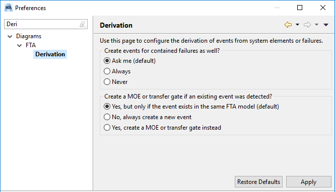
In case an element should be considered as multiple occurring event (MOE) in the fault tree, transfer gates are used and inserted instead of new events automatically. Note that the default behavior is to insert always a MOE event.
Important: There is one exception to the event creation behavior for safety mechanisms: the drag and drop behavior for safety mechanisms will create duplicated events by default. The creation of fault tree events for safety mechanisms is frequently used to model the residual fault, i.e. by ANDing the safety mechanism with a fixed probability of "1-DC" to the detected failure. You can still create a MOE for safety mechanism, but only as a explicit action on the diagram (e.g. drag and drop holding Alt-key down).
By default, the event name and identifier are automatically inherited and kept in-sync as long as they are not overwritten in the event. For example, if an event is inherited from a SysML element, the event name is shown as "[<element name>] failure". For each type element or failure there is a similar rule in place.
In the same manner, the event ID is derived in case the underlying failure has an ID, i.e. malfunctions, failure modes, etc. The derived identifier consists of the prefix "E-" followed by the failure ID. In case the element/failure does not have any identifier, an auto-counter is assigned by default (cp. Auto-counter Patterns).
You can overwrite the event name and ID to adopt it to the appropriate context, either in the diagram or the property sheet. Once overwritten, the name or ID are fixed now to this event and will not be updated any longer from the represented element. To synchronize them again, simply clear the field (i.e. remove the text). Note that the name/ID values are shown in gray color if derived, in black color, if they are overwritten:
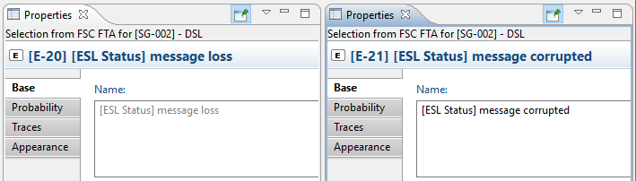
The screenshot above shows a derived name (left side) and an overwritten name (right side).
Instead of recreating an existing FTA model, you can import it from one medini analyze project into another. This can be useful when multiple users develop subcomponents with corresponding FTAs and you want to integrate all the FTAs to evaluate the fault tree at a higher level.
A wizard takes you through the process and includes the option to import connected fault trees. During the import, all events that were linked to elements in the system design to reference failure rates are isolated. The failure rates remain the same but are no longer linked to the elements in the system design. The probabilities in the imported model are calculated based on these isolated events.
Note that while probability parameters from the source model, such as failure rate or repair time, are applied as is, the project settings of the target project may differ from those of the source. This can have an effect on probability calculations. For example, in Risk Time probability models, the Risk Time Interval is applied from the source, but if the target model has different average flight times or mission times, the At-risk time may change.
Custom models are handled somewhat differently. Here, the result is a fixed probability which is calculated based on the mission time of the target project and not the source project. Note that changing the mission time in the target project after import does not change the probability of the imported model.
After you update the source model, you can use the update wizard to update the target model correspondingly. Elements that were modified or deleted in the target model are left as is by default during an update. To restore these to the state of the source model, select the Force Update option during the update. Any elements or traces you added to the imported model are not modified during an update.
Note: You can import the same FTA model to the same project multiple times. The models are listed next to each other in the project. If you selected the Import fault trees... option, connections via transfer gates are preserved in each model.
To import an FTA model, complete these steps.
In medini analyze, open a project and select the folder to which you want to import an FTA model.
Right-click the folder and select Import > FTA from Another Project....
The Import FTA(s) wizard opens.
In the Source Project Selection pane, select the project from which you are importing and click .
In the FTA Selection pane, select all the FTAs you want to import.
Optional. To automatically include connected fault trees, select the Import fault trees connected via Transfer Gates checkbox.
This imports connected fault trees even if you do not select them in the FTA Selection tree.
Click the button.
The Import Results dialog lists the FTA model elements that were added.
Click to complete the import.
The imported model has a imported decorator next to it.
To update the imported FTA model, complete these steps.
In medini analyze, select an imported FTA model.
Right-click the FTA model and select Update FTA....
The Update FTA(s) wizard opens.
In the Source Project Selection pane, the project you previously imported the FTA model(s) from is pre-selected. Click .
In the FTA Selection pane, the models you previously imported are pre-selected.
Note that you cannot cancel the selection of models that were already imported.
Optional. To restore deleted or modified model elements in the imported models, select the Force Update checkbox.
Optional. To automatically include connected fault trees, select the Import fault trees connected via Transfer Gates checkbox.
Click the button.
The dialog lists the updates that were made.
Click to complete the update.
Ansys medini analyze supports qualitative and quantitative analysis of fault trees. In more detail, this means:
Full Fault Tree Evaluation: The quantitative analysis computes reliability metrics such as the top-level unavailability and unreliability, as well as minimal cut sets. For more information about reliability metrics, see Evaluation Results of a Fault Tree.
Minimal cut sets are used in qualitative analysis, which investigates which combination of basic events leads to the top-level event of a fault tree. They can be computed for any intermediate event of a fault tree, not only for the top-level event.
For information about how to evaluate a fault tree in medini analyze, see Full Fault Tree Evaluation.
Probabilistic evaluation: In addition, the diagram editor provides the probability of each event (see Probabilistic Fault Tree Evaluation).
Path Analysis: Path analysis allows to investigate on the cut set fault propagation to the top event through the branches of the tree. The tool provides classical single cut set path analysis, an extended multi cut set path analysis, as well as a quantitative cut set path analysis using heat maps (see Heat Map and Path Analysis).
Combined Cut Set and Design Analysis: The connection of fault trees with design models enables a cut set assessment by following traceability links into (a) the model elements and (b) the failure net of FMEA (see Combined Cut Set and Design Analysis).
To open the Fault Tree Evaluation dialog, right-click an event in an FTA diagram or in the Model Browser and select Evaluate Fault Tree... from the context menu.
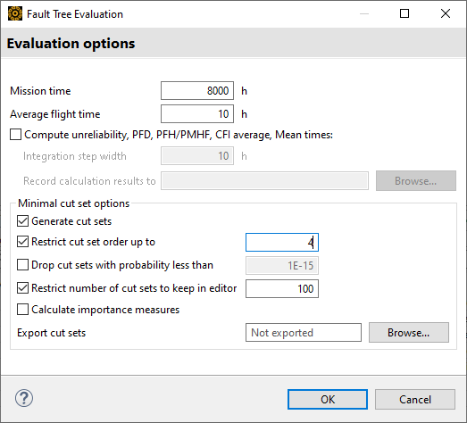
The dialog provides the following evaluation options:
- Mission Time
Determines the interval [0..T] for all time-dependent probability target values and probability distributions. Especially the unreliability (F) is computed for the given interval, unavailability (Q) and event importances are determined for the point in time T (in hours).
- Average Flight Time
Only available in Aviation/Aerospace. Parameterizes the quantitative evaluation for basic events which have the Risk time model. For more information about average flight time in risk time models, see Event Properties and Probability Models.
- Compute unreliability, PFD, PFH/PMHF, CFI average, Mean times
Computes unreliability, PFD, PFH/PMHF, CFI average for the time interval [0..T] as well as mean times.
- Integration Step Width
The mathematical computations above require numerical integrations. Adjust Integration step width for those parameters. For more information, see Evaluation Results of a Fault Tree.
- Record calculation results to...
Records all results of intermediate time steps to a tab-separated text file for further analysis.
- Generate cut sets
Enables the ability to generate cut sets. Clear this check box to save processing time when calculating reliability metrics.
Note that all following options work only when this option is selected.
- Restrict cut set order up to...
Prunes all cut sets that have an order higher than the given number n. Setting this cut-off has no impact on the quantitative top-level computations. Even with no cut sets, you can calculate all other probabilistic target values accurately.
- Drop cut sets with probability less than...
Drops all cut sets for which the worst-case probability at mission time T is below the entered value. For more information, see Minimal Cut Set Results.
- Restrict number of cut sets to keep in editor
Limits the number of cut sets displayed in the resulting table. As with the previous two options, only the cut sets kept in the editor are used to calculate Fussel-Vesely importance, rare event approximation, and Esary-Proschan approximation.
- Calculate importance measures
Enables calculation of the individual event importance measures (Birnbaum, Fussell-Vesely, Criticality). The event importances are influenced by the cut-offs, so that only the set of basic events contained in the cut sets is included in the computation. Note that for larger numbers of minimal cut sets, this can take considerable time.
- Export cut sets
Export batches of cut sets to a specified folder. Enter a folder path in the text field or use the button to navigate to one.
Every one million cut sets are saved in a separate ZIP file. The ZIP files are named in numerical order, beginning with 0.zip. In addition to the ZIP files, an events.csv file is created. It contains the event names and IDs. The IDs help identify the events in the CSV files contained in the ZIP file. The events are identified only by ID to keep the files small.
Note that if you cancel an export while it is still running, medini analyze keeps the already-exported cut sets.
After you have modified the options, click OK to start the evaluation.
The calculation may take a while depending on the fault tree size and the selected cut set order. A high mission time together with a small step width slows down the calculation.
To speed up the calculation, try:
Limiting the number of cut sets. Either restrict the cut set order to small values such as 3 or 4, or restrict the number of cut sets to keep in the editor
Increasing the integration step width
Analysis Results Editor
After successful evaluation, the FTA analysis results editor opens and shows all results.
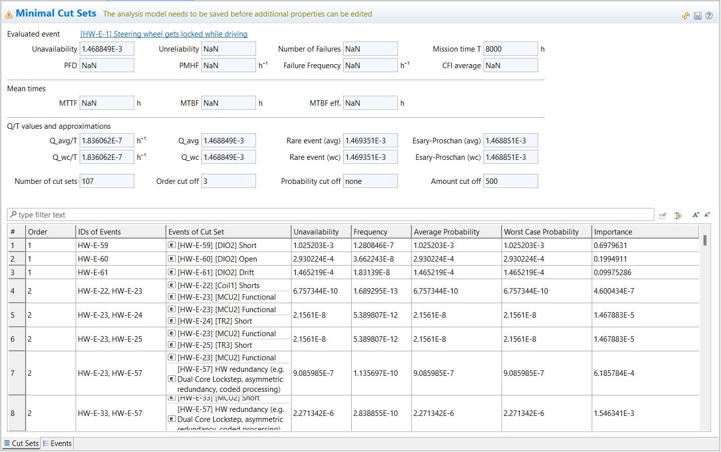
The top section of the model displays the resulting reliability metrics. For more information about how these are calculated, see Evaluation Results of a Fault Tree.
The table in the lower half of the model lists cut sets with a running number, the cut set order ranked by number of events in the cut set, event ID, cut set event names, and four probability values. For more details about these, see Probabilistic Fault Tree Evaluation.
You can now browse, filter, or sort the cut set results as with any other table in medini analyze. You also have the following options:
Table 7.3: Actions in the Results Table
| To... | Do this... |
|---|---|
| ...display the corresponding events in the fault tree diagram |
Right-click a cut set entry and select Highlight Cut Set Events from the context menu. |
| ...display the qualitative path analysis (heat map) |
Right-click an entry and select Highlight events fulfilled by cut set events. For more information, see Heat Map and Path Analysis. |
| ...check which events are part of a cut set | Click the Events tab. In the Events table, the Occurrences column shows the number of cut sets each event is in as a qualitative importance judgement. |
| ...see the importance measures of events | Click the Events tab. In the Events table, the Birnbaum, Criticality, and Fussell-Vesely columns show the different importance measures. For more information, see Evaluation Results of a Fault Tree. |
| ...see cut set statistics such as length counts and total amounts | From the main tool menu, select Window > Show View > Other > General > Error Log. Double-click an entry in the log and read the Message to get more information about the cut sets. |
Important: Cut sets are based on the primary events (node objects) in the fault tree and not the event identifier. For example, if two events with the same ID occur in the fault tree, they are treated as different events. Events are only identical if they are multiple occurring events (MOEs) or referenced with a transfer gate. For more information, see Reoccurring Events. If different events have the same ID, a cut set might appear in the analysis which contains both events, and showing the event ID twice. To prevent such situations, use transfer gates or MOEs. You can also check the Derivation settings for FTA. For more information, see Creation of Events from Models.
For the quantitative fault tree analysis, Ansys medini analyze provides time-dependent evaluations. In addition to a full fault tree evaluation, the tool provides these basic evaluations:
Calculation of top and intermediate event unavailabilities for a given mission time. These probability numbers are shown graphically on the diagram at the events. To trigger the calculation, simply select Calculate Probability from the context menu to update the tree below the selected event (see below).
Quantitative analysis of cut set paths using a heat map. This analysis combines the previous two and allows a graphical inspection of the contributions of different branches in the complete fault tree. For more details see Heat Map and Path Analysis.
Each project manages a global mission time T which is used as default for all computations. However, the tool allows you to selectively override this value for each of the aforementioned evaluations, so that for example a fault tree can be assessed at a different mission time temporarily without affecting all other trees (more precisely: all trees not connected via a transfer). See the following paragraphs for more details.
Probability Update on Diagrams
The quantitative calculation and visualization of probabilities on the fault tree itself (as shown on the diagrams) is triggered from any event by using the context menu:
Right-click an event in an FTA diagram (or Model Browser) and select Calculate Probability... from the context menu. Note that the selected event determines the scope for this calculation.
A dialog opens.
In the dialog, select the computation mode and mission time by selecting one of the following:
Probability at mission time: This option computes a point estimate of the probability at mission time T. All basic events are evaluated at T, and top as well as intermediate events are computed for the same. The probability label thus shows up as P. Note that event latencies are not considered nor might the selected time T be equal to the highest overall unavailability.[5]
Unavailability w/avg. latencies: This option computes the unavailability (Q) by using for each dormant (latent) basic event an average probability. Basically, this is the average dormancy period for MONITORED events (i.e. tau/2). The probability label hence will show up as Q_avg. See Evaluation Results of a Fault Tree for more details.
Unavailability w/worst-case latencies: This option is similar to the above but the unavailability (Q) is computed by taking the maximum dormancy of dormant (latent) events. The probability label hence will show up as Q_wc. See Evaluation Results of a Fault Tree for more details.
The Mission time you enter in the dialog is used for computation. Note that you can override the default mission time, for example, if you want to quickly assess a different time.
Select the check box option in the dialog to also compute and update intermediate event probabilities.
Important: Note that if you do not select a top event, only the subtree below the selected event is updated. The tool allows you to evaluate subtree branches at different mission times. Although this gives you great flexibility for faster analysis of substructures, make sure you have triggered the calculation on the top-event if you want to assess your overall fault tree consistently.
After successful computation, the (sub)tree is updated and the events show the result. If you do not see the probabilty labels, you might have disabled the corresponding diagram option Hide probability labels (button bar above the editor).
Note that this action might also update other fault trees which are connected using transfer gates.
Example
The screenshot below shows an FTA from our example project. To update the probabilities of the complete fault tree, you can trigger the probability calculation in the context menu of an event as shown below:
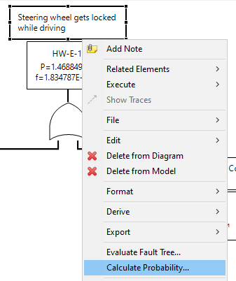
This operation asks for the computation mode (i.e. or average/worst-case unavailability). Select Probability at mission time T for example if you do not have latent events. Note that the mission time is filled by default with the project mission time. If confirmed, the tool updates the event and all intermediate events below so that the probabilities are up to date.
Note that you can also call Evaluate Fault Tree... from any intermediate event node in the tree. In this case, however, the calculation is done only for the subtree starting at that selected event.
The Evaluate Fault Tree... action executes a complete qualitative and quantitative analysis of the fault tree using the options specified, this includes:
Reliability metrics, such as top-level unavailability, unreliability, failure frequency, conditional failure intensity, number of failures, MTTF, MTBF, average and worst-case unavailabilities, and approximations (rare event, Esary-Proschan).
Cut sets including unavailability, frequency, average and worst-case unavailabilities, and cut set importance in relation to the top event
Importance measures for primary events (Birnbaum, Criticality, and Fussell-Vesely) and number of occurrences in cut sets of each event
The subsequent paragraphs provide a detailed description on the computed targets.
The following top event calculations are performed and shown in the editor:
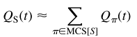
Unavailability: Probability of the top event to occur at mission time T. The probability Q(T) is calculated by the Shannon expansion and conditional probabilities recursively with the formula:

where Ei iterates over all basic events in the fault tree. Note that this value is the exact probability based on the fault tree logic (not an upper or lower bound approximation). If cut set truncation is applied, the accuracy depends on the algorithmic option chosen (see FTA Performance Options).
Hint: The availability of the system follows from the equation: A(t) = 1 - Q(t).
PFD: The Probability of Failure on Demand (PFD) according to IEC 61508 is the arithmetic mean value of the unavailability Q in the interval [0..T]. It is computed based on the following formula:
Unreliability: Probability of the top event to occur in the interval (0..T], namely not including t=0. The unreliability is computed based on the Vesely approximation formula, namely using the conditional failure intensity (λsys):
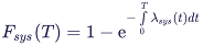
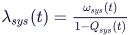
λsys in turn combines the unavailability and the failure frequency w(t), see further below. The precision of the integration is determined by the step width parameter entered in the options dialog for evaluation. Note that from a theoretical point of view that as soon as repairable/monitored events are present, F(t) is only an approximation, since an exact expression for system unreliability of fault trees is difficult to determine in the general case.
Note: By definition, Fsys(0) = 0. You can create fault trees with Qsys(0) > 0, for example by using any of the following:
Fixed probability models
Non-coherent fault trees
Scripted probability models
Weibull distribution with negative time shift gamma
However, in this case it is important to note that, for coherent fault trees, the formula Qsys(t) = Fsys(t) does not hold. Instead, the correct formula is Qsys(t) = Fsys(t) + Qsys(0). The formula Fsys(t) + Qsys(0) can also be used to compute the probability that the top event occurs in [0..T].
Hint: The reliability of the system follows from the equation: R(t) = 1 - F(t). If evaluating an RBD, the R(T) value is computed this way and shown in the RBD diagrams.
PFH / PMHF / Avg. per FH: The arithmetic mean value of the unreliability according to Vesely above per hour in the interval [0..T]. It is computed based on the following formula:
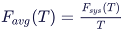
Note that the label of this field varies depending on the project domain profile for Industry, Automotive, and Aerospace. Furthermore, the latest version of IEC 61508 uses also the average number of failures (see Failure Frequency below) as PFH.
Number of Failures: The estimated number of failures of the top level event. The value Wsys is the integral of the failure frequency ωsys(t) (unconditional failure intensity/failure frequency), which is sometimes referred to as Murchland approximation of the system unreliability:
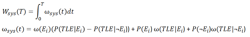
Failure Frequency: Arithmetic mean value of the value ωsys (in the formula above) over the interval [0..T]. The failure frequency is computed as Wsys(T) / T.
Mission time T: The time up to which the evaluation has been calculated. This is the same value as entered in the evaluation options dialog and only here for further reference.
CFI average: Average of the Conditional Failure Intensity (CFI) over the whole mission time. It is computed as the integral of λsys divided by the mission time T.
Mean Time To Failure (MTTF): Mean time to (first) top-level event failure in hours. Note that MTTF is independent of the mission time and computed as follows:

Mean Time Between Failures (MTBF): For repairable and monitored systems, the MTBF value is computed as follows:
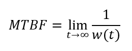
Note that this limes might not always exist, especially for non-repairable systems the MTBF will not be computed and the field shows NaN.
Effective Mean Time Between Failure ("MTBF Effective")[6]: The effective MTBF is a metric that is useful if the overall system is regularly maintained every T hours. That means that if the mission time T is interpreted as just one cycle of operation in the lifetime of the system, this value describes the average time between two consecutive failures and is computed as follows:
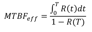
Note that this closed form computation assumes that the system repair time is neglectable compared to T.
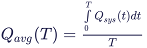
Furthermore, the Q/T values and approximations section provides industry best practice quantities where the unavailability/frequency is computed by considering average/worst-case probabilities of the basic events. The Q/T values are only meaningful if the mission time T is interpreted as an average flight (or drive/cycle) time and latencies are either considered with their average or worst-case exposure times. The following values are computed:
Q_avg: The unavailability using average latencies of all dormant/latent events (via Shannon expansion, see above). Latent events are those that are modelled in one of the following ways:
Use a MONITORED event (i.e. exponential with cycle kind "Monitored") and set the test interval tau larger than the mission time
Use the Risk Time model with a specific time greater than the mission time. If the risk time r_T is less than the mission time, the maximum probability at r_T will be used (hence no difference between average and worst-case)
Note that this Q_avg is hence computed using mean probabilities of the basic events, which is different from the mean of the unavailability Q(t) above.
Q_avg/T: Shows the Q_avg divided by mission time T.
Q_wc: Similarly, this shows a computed unavailability using worst-case latencies of all dormant/latent events. For those events with a test/check interval tau the maximum probability at the end of the test interval will be used, i.e. Pwc(E)=P(tau). The same is true for the Risk Time model with any specific time (less or greater than the mission time).
Q_wc/T: Shows the Q_wc divided by mission time T.
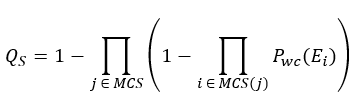
Esary Proschan (avg, wc): The Esary-Proschan upper bound approximation of system unavailability via the cut sets. It uses the average-case or worst-case cut set unavailabilities, i.e. for example the worst-case is computed as follows:
Rare event (avg, wc): Computes an approximation of system unavailabilities via the cut set average/worst-case probabilities:
The minimal cut sets are shown in the table underneath the quantitative targets. The number of computed cut sets will depend on the truncation options choosen, which are shown on the same page (above the cut sets).
For each cut set there are the following values computed (shown in the cut set table):
Unavailability: the cut set unavailability Q(T) at mission time T:

Frequency: the failure frequency w(T) of the cut set at mission time T:
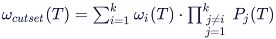
Average Probability: Average cut set unavailability Qavg. This is the product of the average event probabilities, that means Pavg(E)=P(T) for fixed, exponentially distributed, and repairable events, and Pavg(E)=P(tau/2) for monitored and at-risk time events.
Worst Case Probability: Maximum probability of the cut-set, which is given as the product of worst case event probabilities Pwc. These are Pwc=P(T) for fixed, exponentially distributed and repairable events and P(tau) for monitored and at-risk time events.
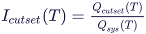
Importance: the cut set importance in relation to the top level event at mission time T:
In addition to the probability and importance of the cut sets the tool also computes event importance measures for the basic events to estimate the relevance of the event. For that purpose the Birnbaum-, Criticality- and Fussell-Vesely-importance measures are calculated and shown on the Events page.
The computations of the measures for an event A are as follows:
Birnbaum Measure: Determines the maximum increase in risk when A occurs compared to when A does not occur:
IB(A) = P{TLE|A} - P{TLE|NOT(A)}
Criticality Measure: Determines the probability that the occurrence of the TLE is a result of an occurrence of A:
IC(A) = IB(A) * P{A}/ P{TLE} = (P{TLE|A} - P{TLE|NOT(A)}) * P{A}/ P{TLE}
Fussell-Vesely: Determines the probability that event A has contributed to the occurrence of the TLE; i.e. it is the ratio of the probability of occurrence of any cut set containing A and the probability of the top-level-event .
Cut set path analysis is an important step in fault tree evaluation, because it allows you to investigate fault propagation across branches in the tree and reasoning about e.g. how safety mechanisms can be effectively added into the design. The tool supports qualitative and quantiative path analysis via a heat map control dialog:
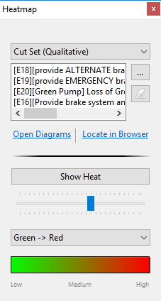
The control dialog will float on top of the all other tool windows. The "type of heat" to show in the diagrams can be controlled via the first drop down field.
To perform a fault tree path analysis follow these steps:
As precondition, the minimal cut sets must be computed and a corresponding editor must be open. Simply calculate the minimal cut sets for a fault tree (or subtree) as described in Full Fault Tree Evaluation and Probabilistic Fault Tree Evaluation.
To bring up the path analysis heat map control choose either:
Highlight events fulfilled by cut set events: This will start a qualitative path analysis from the cut set list. The dialog will automatically select Cut Set (Qualitative) as heat type which will color the fault tree paths from the selected cut set up to the Evaluated event for which the cut sets have been computed.
Show heat of cut set path: The dialog quantitative path analysis will color the gates and intermediate events along the path up to the Evaluated event according to their probability contributions (relative to the selected cut sets). See the example below for more information.
Select Open heat map control dialog from the top button bar. Afterwards, choose the kind of heat and select the cut sets from any open cut set editor using the "..." button
Use the Open Diagrams link to bring up the fault tree or navigate to the Model Browser and open a fault tree diagram for inspection
Click Show Heat to turn on the coloring in the diagrams. The slider below adjusts the transparency of the colors. Optionally, select a different color spectrum.
Use the "..." button to select a different cut set to switch between different result entries
Note that both qualitative and quantitative cut set heat maps allow the selection of multiple cut sets or a complete cut set result model (i.e. all cut sets). For example, you can select all single or dual point faults and visually check how they propagate through the fault tree, or inspect which branches have been truncated from the evaluation due to cut set order cut offs. A more sophisticated example of quantitative path analysis is shown below.
The cut set (path) analysis can be continued into an underlying SysML design model or failure net. If a SysML diagram is opened for which a fault tree event is in a cut set, the corresponding element will be colored as well. The same is true for the graphical dependency/failure net editor. Please refer to Combined Cut Set and Design Analysis for more details.
Example
Consider the ESL example project that is shipped with the tool. Evaluating a quantified fault tree allows the selection of a complete analysis model, i.e. effectively all events:
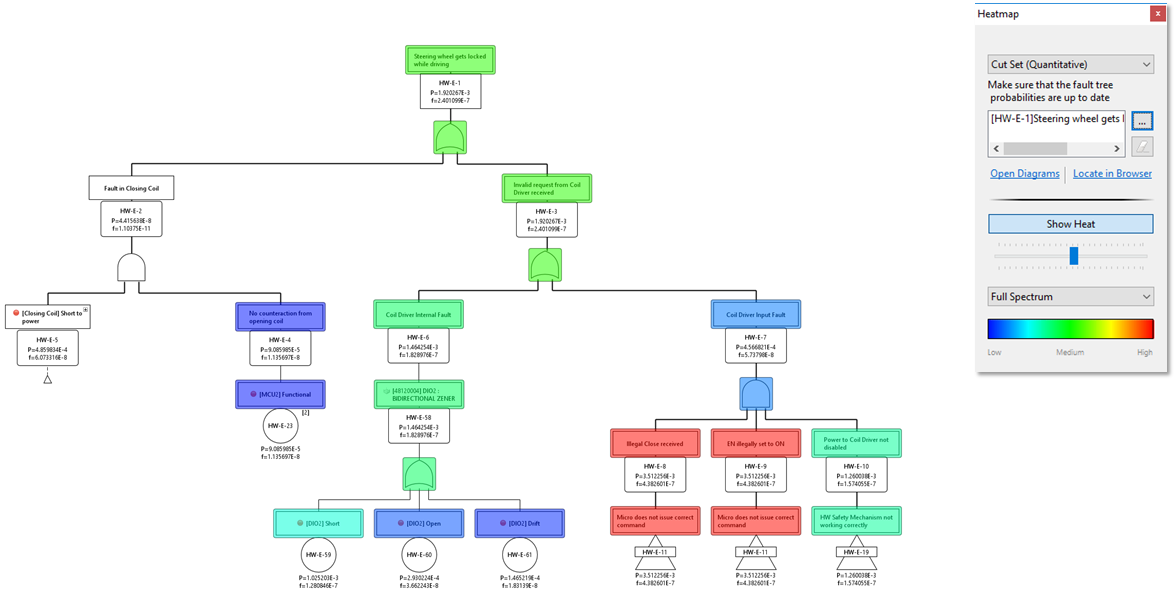
The screenshot shows the heat distribution over various branches of the fault tree. The heat coloring indicates the relative contributions of the intermediate events/gates to the top event. As can be seen, the hot paths are two branches on the right side which are "cooled" by the AND gate. This provides for example a visual feedback on the importance of the mechanism behind an AND gate.
Note that events which are not colored at all ("transparent") are not part of any cut set. In this case, the branch on the left is a "dead" subtree: none of the cut sets will contribute via this path to the top event! This means either a cut set order truncation has been applied or the paths are by-passed by e.g. a MOE.
The connection of fault tree events with failures/components in the design model allows a detailed assessment on where events appear and whether they are e.g. at risk of not yet considered common causes or cascading failures. For this purpose, the FTA component supports the graphical inspection of cut sets in a connected SysML model or failure net.
To analyze cut set events in connected models you can do the following:
Evaluate a fault tree to compute its cut sets, either qualitatively or quantitatively (see Full Fault Tree Evaluation and Probabilistic Fault Tree Evaluation)
Open the heat map control dialog (see Heat Map and Path Analysis)
Open either the failure net of any event or a SysML diagram for a component for which its failure modes are represented in the cut set.
If any of the elements in the diagram has a representation in the selected cut set(s) or the paths up to the top event, the element will be colored. Since elements can have multiple failure modes/malfunctions, the containing element will be colored as soon as a single failure is part of a cut set path.
The failure net will color all cause-effect chains upwards for the selected cut set (or intermediate events representing a failure)
Examples
Let's assume a cut set event references a failure mode "AMP1: Functional failure". Opening the failure net editor on any failure in the cause-effect chain developed along an FMEA will be highlighted. For example, the failure in focus in the following screenshot is "No Lock State Information" of the ESL Controller element (middle):
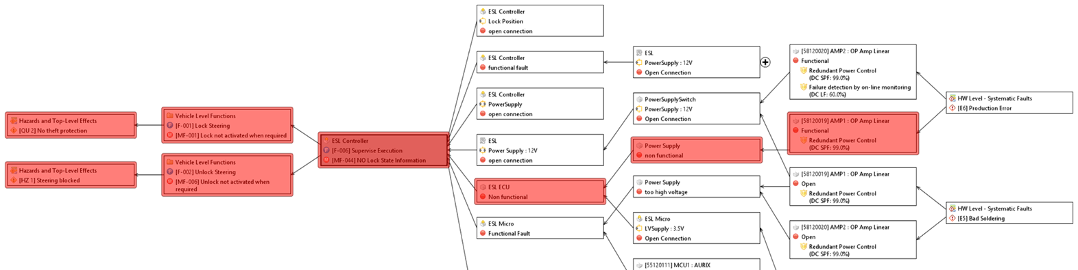
Since the AMP1 failure is an indirect cause to this failure, the failure net path will be highlighted accordingly. Note that this highlighting is independent of whether the failure in focus or any other failure along the chain is actually part of the fault tree!
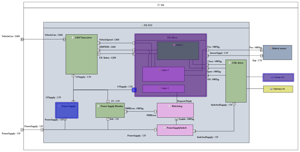
Another example could be the selection of the complete quantitative cut set analysis. The following screenshot shows the parts that are (a) covered by the fault tree and (b) how they contribute relatively to the top event:
The FTA module is capable of handling common cause events in an explicit way during qualitative and quantitative analysis of a fault tree.
A common cause analysis is especially important if redundancy is used to reduce the overall probability of the system failure. In such cases, it is important to understand what are the common causes (single events) that can lead to a simultaneous (at the same time or nearly the same time) failure of system parts or components that have been considered as being independent and redundant. There can be multiple sources for common cause failures such as:
common mistakes in maintenance procedures
common environmental conditions, that can affect multiple systems at the same time
material or production problems that affect multiple components or parts
The common cause failures have to be modeled explicitly as events in the fault tree (compare e.g. NUREG/CR-4780). They are an example for multiple occurring events which are modeled in medini analyze using transfer gates or MOEs. Assuming the example fault tree below, we have three independent components each with a probability of 0.01 which calculates to a TLE probability of 0.000001 due to the AND-gate.
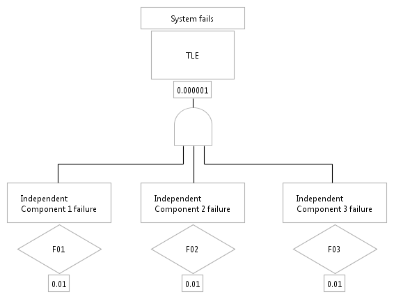
If there is a common cause failure, that could lead to a simultaneous failure of all three components, this event has to be explicitly modeled in the fault tree like in the example below.
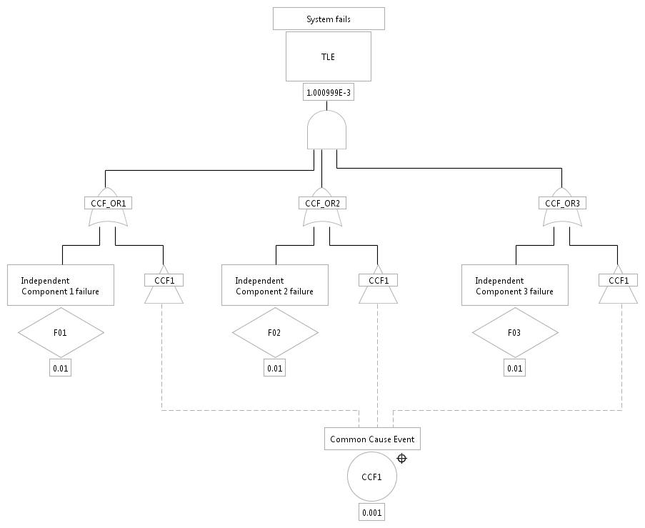
As to be seen, the event "Common Cause Event" with identifier "CCF1" has a probability of 0.001. It is added via an OR-gate and transfer gates to all three independent components.[7]The overall probability of the TLE is now calculated to 0.001000999. Note that it is not necessary to place the common cause event on the same diagram: it can reside even in a separate fault tree model.
The FTA algorithm in the tool is designed to handle fault trees with a large number of gates and events. Since the inherent complexity to solve fault trees can lead to low performance in specific cases, the tool features two algorithmic options for fault tree evaluation that can be modified under Window > Preferences... > Diagrams > FTA > Evaluation[8]:
BDD based computations (default). The fault tree is solved in the most accurate way using latest state of the art techniques such Binary Decision Diagrams (BDD). These techniques provide exact quantitative results for all probability calculations (i.e. unavailability, unreliability, etc.), independent of cut set truncations. This means that any truncation of cut sets selected in the evaluation, such as the number of events in a cut set or probability thresholds, does not affect the quantitative results.
Note that some rounding errors due to approximation errors in numerical integration or rounding errors in floating point operations may occur.
While this option provides the exact results, it consumes more memory and runtime than the next option described below.
Cut set based computations. Typically, fault trees are solved by computing cut sets first and derive the quantitative targets such as unavailability from these sets. This approach provides usually the fastest results, if truncations are used (i.e. order of cut sets and probability threshold). By using cutoffs, however, the quantitative results will be affected by the cut offs and the results need to be approximated based on the remaining cut sets.
If this option is selected, also the probability computations on diagrams will use the same approach (see Probabilistic Fault Tree Evaluation). Therefore, you can specify additionally a Truncation order for intermediate events that will perform cut set truncation for any subtree below an intermediate event.
If you experience performance problems in the FTA computations, you can change the evaluation option to Cut set based (option 2) and follow these steps to get the best results:
Go to the top event you want to evaluate and perform "Evaluate Fault Tree...". In the options dialog select "Restrict cut set order" and select 3. Press OK to start the evaluation.
If the fault tree solving is fast, you can re-evaluate the fault tree and increase the cut set order stepwise. Depending on the tree structure, usually you will not need an order higher than 6 to receive accurate estimations, unless you have AND/Voting gates with a larger number of inputs/threshold.
Note that you can keep the analysis editors open while you increase the stepsize (if cut set size is reasonable and enough memory is present). This allows you to compare the quantitative approximations. In most cases the quantitative results are already with smaller cut set order very close so that increasing the cut set order will not lead to more accurate results.
If you still have too many cut sets and the result editor takes very long to open, you can apply a probability cutoff to reduce further the number of cut sets.
In case you perform "Calculate Probabilities..." on diagram, always first try without selecting intermediate event probabilities in the options dialog. If this works fast enough, you can enable the computation of intermediate events as well.
In case the "Calculate Probabilities..." is slow, go back to the Preferences and decrease the number in Truncation order for intermediate events. Reducing this number will increase the performance, but the results will loose precision.
Important: Note that in case the truncation order is less than the number of inputs to an AND gate, the probability might result in P=0.0 for some subtrees (i.e. the intermediate event above the AND). This happens due to the elimination procedure so that if P=0.0 effectively means that the number of cut sets considered for this gate are empty. The same applies to Voting Gates with a threshold number higher than the cut off. However, this value does not mean that the events below are not considered for the overall top probability, since events might contribute via transfer gates to different intermediate events and paths to the top.
Basically there are two copy functionalities available for fault trees:
Copy and paste of whole FTA models inside the same project. This operation will preserve all relationships, especially to elements of design models that are used as source for probability/failure rate numbers.
Copy and paste of events, gates, and sub-trees in the same or across projects. This operation will preserve relationships dependent on the target model. If the target FTA model is inside the same project, all relationships will be preserved. If parts of a fault tree are copied to another project, these elements will be inserted as a "self-contained copy" of the original elements. That means e.g. references to system design elements are released, but probability/failure rate data will be preserved as far as possible (details see below).
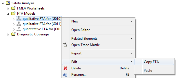
Copy and paste of whole FTA models can be triggered via the context menu of the Model Browser. If a fault tree model is selected, the context menu contains the entry "Edit -> Copy FTA" to initiate the operation.
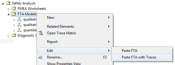
After selecting copy paste is supported within the same project. For this purpose the "Edit" sub-menu in the context menu of any package below "FTA Models" will show two paste entries: "Paste FTA" and Paste FTA with Traces". The former option will create an exact copy solely of the FTA model in the selected folder, while the latter will in addition establish traces to copied fault tree nodes, whenever a trace from another element in the project exist into the fault tree. For example, if a trace from a safety goal to the top level event exists, a trace will be created to the copy of the top level event as well.
Hint: A duplication of whole FTA models is also available by drag and drop in the model browser while holding the "Ctrl"-key pressed. In this case the target package for the copy can easily be selected during the drop (release of mouse button). A dialog will pop up asking whether traces shall be copied or not.
The copy of individual events, gates or sub-trees can be triggered directly within the graphical editor using the context menu (cp. General aspects for graphical editors).
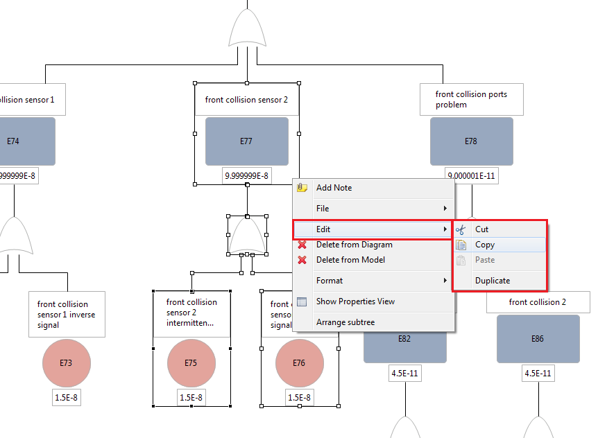
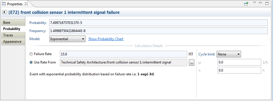
The copy operation will try to preserve any probability settings of the copied events. In case the event is pasted into another project, but uses a system design element to derive it's failure rate/probability, the event's properties will be encapsulated to maintain the same probability semantics. For example, if an event is derived from a failure mode "intermittent signal" that has a failure rate of 15 FIT, the failure rate information will be copied into the event as shown below.
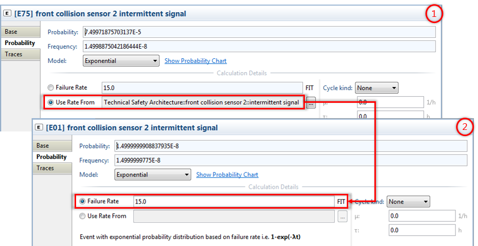
The copy loses the reference to the design element and hence "Derived failure rate" will be automatically changed to the fixed failure rate at the event.[9]Note how this might lead to a change in the event probability in case the mission time at the target FTA model is different. In the example shown above, the mission time at the source model is set to 1h, whereas the mission time of the target model is set to 30h. As consequence, the calculated probability is adapted accordingly.
Important hint: the copy operation copies the failure rates at the moment when the copy/paste is executed. That means in case the failure rates have been defined over a failure rate catalog/formula and mission profile, you should make sure the numbers are up to date. If unsure, execute a "Re-compute failure rates" on the whole project. For details see also SysML Blocks: Facilitating the type concept.
Transfer gates to events that are not in scope of the copy operation will be handled similarly, if copied into another project. For example, if a transfer gate is pointing to a target event in a another model, the copy will have no target event set. This is only the case if the copy happens inside the same project, or if the target event is copied together with the transfer gate.
Fault tree results might lead to a refinement of the system design and contribute new (safety) requirements. The latter is supported via the Derive context menu of an event. To derive a new safety requirement choose "Derive Requirement..." as shown below.
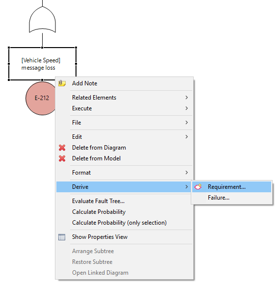
In the upcoming dialog select the target safety requirements model where the new safety requirement shall be inserted. After confirming the creation a new safety requirement appears with the name of the event and a back-trace to the event of the fault tree.
Fault tree results may reveal new failures in the system design or find similar or same failures, already found by other means. The quick derivation or linkage of failures is supported via the Derive context menu of an event. Choose "Derive Failure..." as shown below in both cases.
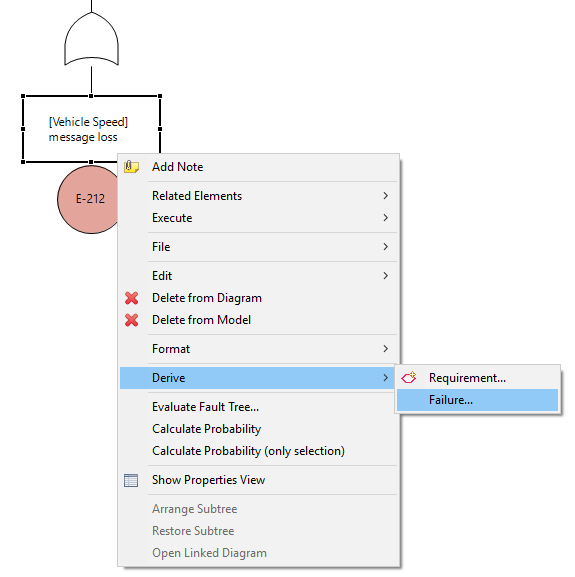
In the upcoming dialog either select the target element or failure collection to create a new failure or select any existing failure. In both cases, the failure is linked to the element afterwards, except if you choose not to do so by checking the Do not link failure with event option in the dialog.
Note that the derivation of failures supports multi-selection. So in case you have multiple events selected, a new failure for each of the selected events is created. Linking to existing failures is not supported in this multi-selection case though.
Another note: if you link an FTA event to an existing failure, the tool will ask you, whether you want to overwrite the failure's name with the event name and keep them in sync after that) or whether you want to keep things as they are.
[5] This computation mode has been the only available for diagrams in earlier versions than 2022 R1.
[6] Sometimes also referred to as MTBF with scheduled replacements, see e.g. https://www.weibull.com/
[7] Note that since V2.5.0 the modeling of events with the same ID is no longer supported, since it easily lead to inconsistencies in events expressing the same cause. The former constraint error #31 is now only a warning, since multiple events with the same ID are treated as different events.
[8] The algorithmic choice is also applied to RBD which use the same core engine in the tool.
[9] Note that this will also happen in case the target project contains the same System/Function Model element/failure rate provider.