Linear buckling analysis can be used for estimating the critical load, or bifurcation load, of a stiff structure. This is done by solution of the generalized eigenproblem:

where Kg is the geometric stiffness matrix (due to stress stiffening effects) and Km is the material tangent stiffness matrix. To compute Kg, loading must be applied to the structure so that stresses develop. For the numerical solution to work well, the applied loading should be high enough to result in a well-defined geometrical stiffness matrix, compared to the tangent stiffness. The pre-loading can be applied by a static implicit analysis.
Linear buckling analysis is activated by using the keyword
*CONTROL_IMPLICIT_BUCKLE. A linear buckling analysis may be part of a
linear or nonlinear static analysis. Linear (eigenvalue) buckling is a linear procedure,
with all the limitations mentioned in Linear Static Analysis.
This means that contacts will not be updated and that material responses are linearized.
Plasticity is not considered during the buckling phase.
A template for linear buckling analyses follows:
*KEYWORD
.
.
.
*INCLUDE
database_cards_static.key
*CONTROL_TERMINATION
        Define end time of the simulation
*CONTROL_IMPLICIT_BUCKLE
        Define parameters for buckling load evaluation
*INCLUDE
        Include file defining geometry, materials etc.
*LOAD_...
        Define nodal loads etc.
*BOUNDARY_...
        Data line to prescribe boundary conditions
*TITLE
        Simulation title
*END
By default, the buckling analysis will be performed at the termination time of the simulation. However, you can perform intermittent buckling analyses at different stages of the simulation. A curve ID can be specified by entering the LCID as a negative number. The x-values of the curve specifies at which time(s) the buckling analyses are to be performed. The corresponding y-value specifies the number of buckling modes to compute. An example based on a nonlinear implicit pre-loading of a structure is given in Linear Buckling Analysis of a Panel With a Bead.
Buckling load factors are printed in the eigout file. The
buckling load is simply the eigenvalue times the applied load. The buckling mode shapes
are output in the d3eigv file(s). To get output of stresses in the
d3eigv file(s), include
*CONTROL_IMPLICIT_EIGENVALUE with NEIG = 0 and
MSTRES = 1.
Note: A linear buckling analysis may severely overestimate the physical buckling load of a real-world structure. It neglects nonlinear effects (plasticity, failure, large deformations) and imperfections.
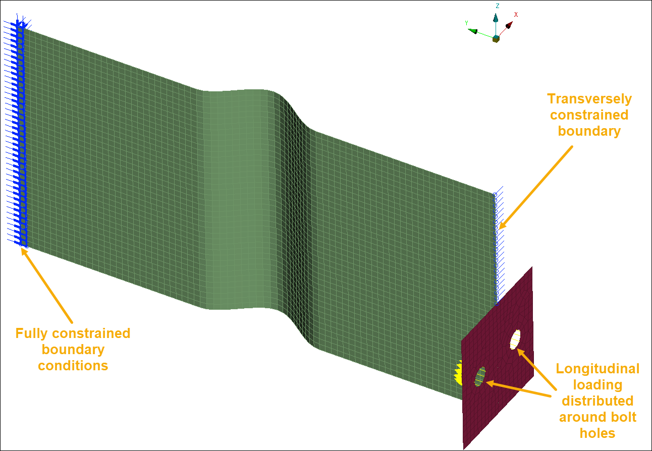
A panel is fully constrained at one edge and loaded by a force distributed around the bolt holes in the flange, as shown in the following figure. The edge at the flange is constrained in the transverse direction. The example keyword file is buckle001.key.
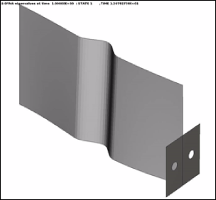
First, a pre-loading of 32 kN is applied in a nonlinear implicit analysis, then a linear buckling analysis is performed. The lowest eigenvalue is 12.078, corresponding to a buckling load of 386.5 kN. The buckling mode shape is shown below.