


The first step in running a simulation with Offshore capabilities is to add an Ocean Environment object to the analysis. Once the Ocean Environment is added, you will be able to add other Offshore-specific objects. For a Harmonic Response analysis, you should set the Analysis Settings Solution Method option to Full.
You can only have one active Ocean Environment object in an analysis. Additional Ocean Environment objects may only be created once any existing Ocean Environment objects have been deleted or suppressed.
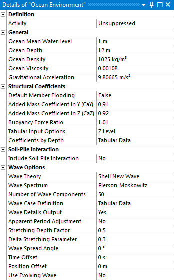
The Activity field allows you to set the suppression state of the Ocean Environment object. Set it to Suppressed if you want to exclude the object from the analysis.
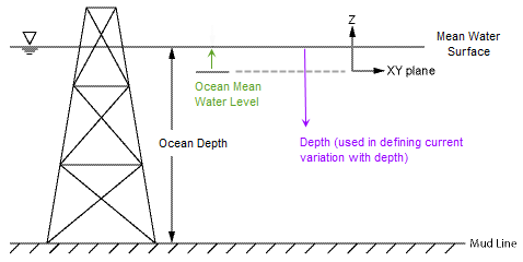
The ocean geometry is defined by the Ocean Mean Water Level (mean water surface Z position with respect to the global origin) and the Ocean Depth (vertical distance from the Ocean Mean Water Level to the seabed).
The material properties of the seawater are defined by the Ocean Density and Ocean Viscosity. The latter is only used where the global structural coefficients are set to vary by Reynolds number (see Structural Coefficients). The default values of Ocean Density and Ocean Viscosity are set to 1025 kg/m³ and 0.00108 Pa s, respectively, which are applicable for seawater at a temperature of 20°C and a salinity of 0.035 kg/kg.
The vertical acceleration due to gravity is defined by the Gravitational Acceleration property, which defaults to the standard value of 9.80665 m/s².
These coefficients apply to all submerged line bodies in the Geometry.
Default Member Flooding controls whether tubular line bodies are considered to be flooded by the surrounding seawater or not. (An internal fluid for tubular line bodies can also be defined with Component-Based Variation or Pipe-in-Pipe objects.)
Added Mass Coefficient in Y (CaY) and Added Mass Coefficient in Z (CaZ) control the ratio of added mass to displaced mass, where the added mass is the mass of seawater that moves with the line body in a dynamic analysis, in the two directions perpendicular to the line body axis.
Buoyancy Force Ratio can be used to adjust the buoyancy of line bodies relative to the buoyancy force based on the line body displacement and the defined Ocean Density. This may be useful when accounting for external pipe features that are not explicitly modelled.
Drag and inertia coefficients are also defined for all submerged line bodies. These coefficients can be set to vary by vertical Z position, or by the Reynolds number of the relative fluid flow around the line body; set Tabular Input Options to Z Level for the former, or Reynolds Number for the latter.
Depending on your selection, you can then set Coefficients by Depth
or Coefficients by Reynolds Number using the tabular data input. The
independent variable is entered in the first column, followed by the Drag Coefficient
in Y (CdY), Drag Coefficient in Z (CdZ), Drag
Coefficient in X (CtX), Inertia Coefficient in Y (CmY) and
Inertia Coefficient in Z (CmZ). All coefficients are defined in the local
line body axes. Click the  icon to add more rows to the table. Duplicate entries of Z Level or
Reynolds Number are ignored.
icon to add more rows to the table. Duplicate entries of Z Level or
Reynolds Number are ignored.
Note: At least one row of tabular data must be defined.
The values for CaY/CaZ will be used as defined; there is no assumption that Ca = Cm - 1.0.
You can choose to Include Soil-Pile Interaction. Setting this option to Yes allows you to specify a Soil-Pile Data File, which may be a Mechanical APDL macro (.mac) file or some other APDL code snippet. The specified file is included in the solver input file via the /INPUT command.
Examples of soil-pile interaction macros may be obtained through a Service Request on the Ansys customer site.
The following options are used to define wave and current conditions for the simulation.
Wave Theory
In Static Structural and Transient Structural analyses, you can define a Wave Theory to be used in the calculation. The available options are:
No Water Motion: no fluid motion will be accounted for in the calculation
Current Forces Only: no wave motion will be accounted for, but the effect of an Ocean Current may be included
Airy: small amplitude first-order periodic wave
Wheeler: Airy wave with Wheeler stretching to account for the variation of water depth with wave surface
Stokes: fifth-order wave theory for periodic waves in intermediate or deep water
Stream Function: stream function wave theory suited to periodic waves in shallower water
Random: a random, but repeatable, non-periodic combination of Airy waves fitted to a selected wave spectrum
Shell New Wave: similar to a random wave, but with a modified surface coefficient to better represent the most probable maximum condition of a real sea
Constrained: embeds a Shell new wave into a random wave
Diffracted: allows pressures and motions to be imported from a Hydrodynamic Diffraction analysis
User Defined Wave: calls the Mechanical APDL subroutine userPartVelAcc for the input of user-defined wave and current information
A more complete description of these wave theories is provided in Hydrodynamic Loads in the Mechanical APDL Theory Reference .
In a Modal analysis, or where the imported Geometry contains only solid bodies, water motion is not permitted. In a Harmonic Response analysis, the wave information is entered via the Harmonic Wave Load object. Harmonic Response analyses are restricted to periodic waves (Airy, Wheeler, Stokes, Stream Function or User Defined Wave).
For Static Structural and Transient Structural analyses, if the imported Geometry does not contain any line bodies but does contain surface bodies, you can only choose between No Water Motion or Diffracted. If the imported Geometry does contain line bodies, you are free to select from any of the wave theories listed above.
Wave Spectrum
Where the Wave Theory is selected as Random, Shell New Wave or Constrained, an additional Wave Spectrum option is shown. This is used to select a wave spectrum to which the combination of linear waves is fitted. The available options are:
Pierson-Moskowitz: a formulated spectrum defined by peak wave period and significant wave height
JONSWAP (Joint North Sea Wave Project): a formulated spectrum defined by peak period, significant wave height and a peak enhancement factor
User Defined: an unformulated spectrum defined by the frequency/spectral energy density data in a User Defined Spectrum object
Wave Case Definition
For any Wave Theory other than No Water Motion, the Wave Case Definition tabular data input is used to define the current and/or wave properties for the calculation. The number of rows in the Wave Case Definition table will match the Number of Steps defined in the Static Structural or Transient Structural Analysis Settings; a separate load case may be defined for each step of the analysis.
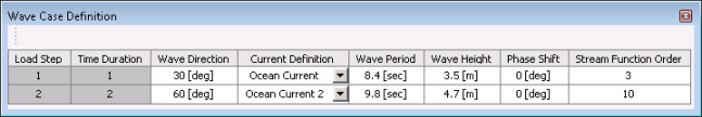
All wave theories require a Current Definition at every step. Use the drop-down menu to select from any of the Ocean Current objects that you have defined in your analysis, or choose Disable Current to exclude current effects for that step.
For all wave theories that include wave motion, a Wave Direction may be defined at each step. This sets the direction that the incident wave travels towards, relative to the direction of the global X axis.
For wave theories of Airy, Wheeler, Stokes, Stream Function, Diffracted and User Defined Wave, the wave properties are specified by the Wave Period, Wave Height and Phase Shift. Setting the Wave Period or Wave Height to zero will disable the wave motion for a given step. For a Stream Function wave, the Stream Function Order may also be defined; for a User Defined Wave, the Wave Length may be defined.
For Random, Shell New Wave and Constrained waves, the wave property definitions depend on the selected Wave Spectrum. These are summarized in Table 1.
Table 8.1: Wave Properties for Non-Periodic Wave Theories
| Wave Spectrum | ||||
| Pierson-Moskowitz | JONSWAP | User Defined | ||
| Wave Theory | Random |
Peak Period Significant Wave Height |
Peak Period Significant Wave Height Peak Enhancement Factor | User Defined Spectrum |
| Shell New Wave |
Peak Period Max Wave Crest Amplitude |
Peak Period Max Wave Crest Amplitude Peak Enhancement Factor | User Defined Spectrum | |
| Constrained |
Peak Period Significant Wave Height |
Peak Period Significant Wave Height Peak Enhancement Factor | User Defined Spectrum | |
Where applicable, in the User Defined Spectrum column of the Wave Case Definition table, you should use the drop-down menu to select from any of the User Defined Spectrum objects that you have defined in your analysis.
Additional Options
For periodic waves (Airy, Wheeler, Stokes, Stream Function or User Defined Wave) the Force Application option allows you to set the position/orientation of elements relative to the wave surface for the force calculation. The available options are:
Act on Elements at their Actual Location
Use Wave Peak: elements are assumed to be positioned at the wave peak
Use Wave Trough: elements are assumed to be positioned at the wave trough
Vertical Upward Force Only
Vertical Downward Force Only
The Wave Details Output option indicates that a description of the defined wave should be written to the Solution Information. For non-periodic waves, this includes details of the wave components.
For Airy, Wheeler, Stokes and Stream Function waves, the MacCamy-Fuchs Adjustment option allows you to include or exclude a correction to the structural inertia coefficients to account for diffraction effects. This is relevant for larger diameter line bodies in shorter wavelength waves.
For Random, Shell New Wave and Constrained waves:
The Number of Wave Components allows you to set the number of constituent waves for the wave combination
The Apparent Period Adjustment option allows to you include or exclude a calculation of the apparent period where a wave is superimposed over a current
The Stretching Depth Factor is used to provide the wave kinematics under the wave crest, in a form of Wheeler stretching known as delta stretching
The Delta Stretching Parameter sets the shape of the delta stretching function
For Random and Constrained waves:
The Wave Kinematics Factor is used to account for wave spreading by modifying the horizontal wave kinematics, where a value of 1.0 corresponds to no spreading
The Initial Seed sets the seed for random phase angle generation
For Shell New Wave and Constrained waves, the Time Offset and Position Offset set the time and position offsets at which the maximum wave crest will occur.
For Shell New Waves the Wave Spread Angle is used to compute a wave spreading factor to modify the horizontal wave kinematics for near-unidirectional seas, while the Use Evolving Wave option may be used to modify the component wave phase angles over the simulation.
Where the Wave Theory is set to Diffracted, additional pressure mapping options are displayed. Use the Hydrodynamic Data File selection dialog box to choose an Aqwa-generated hydrodynamic database (.ahd) file, which will be used to determine hydrodynamic loads on line body elements. Where the imported Geometry includes surface bodies, use the Scoping Method and Geometry/Named Selection options to define the surfaces onto which the hydrodynamic pressures will be transferred.