


This section demonstrates how to use Ansys Polymat to perform non-automatic fitting.
Start Ansys Polymat by typing polymat, as described
in Starting Ansys Polymat. You will use
the Ansys Polymat graphical user interface (which is described in User Interface) to set up your model.
Click the  curve button to open the Create a New
Curve dialog box (Figure 1.4: The Create a New Curve Dialog Box).
curve button to open the Create a New
Curve dialog box (Figure 1.4: The Create a New Curve Dialog Box).
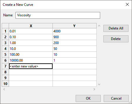
Enter Viscosity for Name; this
will act as the name of your data curve. Next, enter the coordinates of each of
the 6 data points listed in Problem Description in the appropriate X and
Y column of each numbered row, as shown in the previous
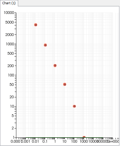
figure. Finally, click to close the dialog box and
plot the data points in the chart.
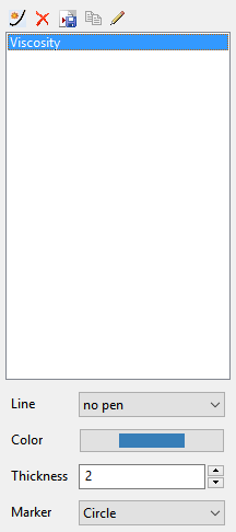
The curve list (Figure 1.5: The Curve List) will now contain a single curve: Viscosity.
Next, in order to fit a model to your experimental data curve, you will select the curves to be calculated. In this case, it is just the shear viscosity curve that is to be fitted, but in other cases you will usually have multiple data curves available.
Click the Rheometry menu button (located near the top left side of the application window) to open the Load Curves (Part I) menu. The Shear Viscosity curve is selected by default, so you can simply select Upper level menu to return to the main menu.
There are several parameters you can modify to control the calculation of the model curves. Click the menu button to open the Numerical Parameters menu. For this example, you will keep the default settings (log-log plot, 100 data points, and so on), so you can simply select Upper level menu to return to the main menu. See Defining Numerical Parameters for details about these parameters.
To define the type of fluid model you want, select the Select Fluid Model menu item in the Ansys Polymat menu.
![]() Select Fluid Model
Select Fluid Model
The default selection is for an isothermal Generalized Newtonian model, so you can simply select Upper level menu to return to the main menu.
Now you can choose the power-law model and set initial values for its parameters. In the Ansys Polymat menu, select Material Data.
![]() Material Data
Material Data
Then choose Shear-rate dependence of viscosity.
![]() Shear-rate dependence of viscosity
Shear-rate dependence of viscosity
In the resulting menu, select Power law.
![]() Power law
Power law
As described in Power Law, the viscosity η depends on
the shear rate  as follows in the power law:
 | (1–1) |
The parameters K, λ, and
n are called, respectively, fac,
tnat, and expo in the
Ansys Polymat interface. Each has a default value of 1. The parameter
K corresponds to the shear viscosity obtained at a
shear rate  . In view of this, the same viscous behavior can be described
by means of various sets of K, λ pairs.
. In view of this, the same viscous behavior can be described
by means of various sets of K, λ pairs.
Before doing any fitting, you need to estimate the minimum and maximum shear rates occurring in the flow being simulated. You will try to fit the power-law model to the experimental curve in that range of values. For this example, the minimum and maximum shear rates are considered to be 0.1 and 10 s-1.
As a first step, you will try to determine the value of K
that matches at least one experimental data point, say, at a shear rate of 1.
For this, consider λ=1 and n=1
(the default values). λ has been taken as the inverse
of the selected shear rate,  , so that the argument of the power law is 1. You will change
the value of K until the viscosity curve matches the
experimental data at the point (1, 200).
, so that the argument of the power law is 1. You will change
the value of K until the viscosity curve matches the
experimental data at the point (1, 200).
First, try keeping K=1 (the default value). Click the menu button. Ansys Polymat will use your initial values to compute a shear viscosity curve; this computed curve will then be drawn in the same chart that displays the experimental data points you added previously.
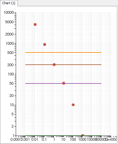
Now you can try other values of K and have Ansys Polymat compute the viscosity curves for those values.
To modify the value of K, click the Modify fac menu item in the Ansys Polymat menu and set the new value using the dialog box that opens.
![]() Modify fac
Modify fac
Set K=50, and click the menu button to update the chart with the new curve. Repeat for K=500 and K=200. Figure 1.7: Computed Viscosity Curves for Various Values of K shows all of the curves for the various values of K. The curve for K=200 matches the point (1, 200), so this is the value you will keep for K.
Now that you have determined the best value for
K, you can begin to determine the best value for
n, keeping K=200 and
λ=1. Changing the value of
n will rotate the computed curve around the
point  .
.
To modify the value of  , click the Modify expo menu item
in the Ansys Polymat menu and set the new value using the dialog box
that opens.
, click the Modify expo menu item
in the Ansys Polymat menu and set the new value using the dialog box
that opens.
![]() Modify expo
Modify expo
Try setting n to 0.7, 0.5, and 0.3, and click the menu button to update the chart with the new curve after each change in n. Figure 1.8: Computed Viscosity Curves for Various Values of n shows all of the curves for the various values of n. The curve for n=0.3 matches the experimental data (in the range from 0.1 to 10 s-1), so this is the value you will keep for n.
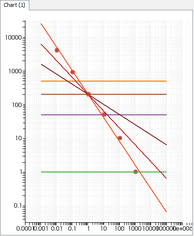
Thus the fitted values of the parameters are K=200, n=0.3, and λ=1. A change in λ will necessarily lead to a change in K.
Once you are satisfied with the parameters, you can save them to a material data file. Click Upper level menu three times to return to the top-level Ansys Polymat menu. Then click Save in a Material Data File.
![]() Save in a Material Data File
Save in a Material Data File
In the resulting dialog box, specify a name for the material data file (e.g.,
sample.mat) and click .
When asked if you want to define or check the system of units, click
.
Since you are going to be using the same experimental data to practice using the automatic fitting method, it will save you some time if you can reuse these experimental data, instead of redefining them.
To save the experimental data, first select the Viscosity
from the curve list on the right side of the application window. Then click the  curve button, which is located above the curve list. In the
dialog box that opens, specify a name for the curve file
(
curve button, which is located above the curve list. In the
dialog box that opens, specify a name for the curve file
(sample.crv) and click .