


There are currently 10 laws available for  , plus the default constant value.
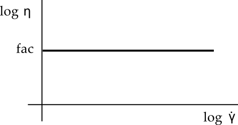
For Newtonian fluids, a constant viscosity
 | (6–7) |
is the default setting.  is referred to as the Newtonian or zero-shear-rate viscosity,
and its default value is 1.
is referred to as the Newtonian or zero-shear-rate viscosity,
and its default value is 1.
The units for  and its name in the Ansys Polymat interface are as follows:
| Parameter | Name in Ansys Polymat | Mass | Length | Time |
|---|---|---|---|---|

| fac | 1 | –1 | –1 |
Figure 6.3: Constant (Shear-Rate-Independent) Viscosity shows a plot
of a constant  .
.
The Bird-Carreau law for viscosity is
 | (6–8) |
| where |

| = | infinite-shear-rate viscosity |

| = | zero-shear-rate viscosity | |

| = | natural time (that is, inverse of the shear rate at which the fluid changes from Newtonian to power-law behavior) | |

| = | power-law index |
The units for the parameters and their names in the Ansys Polymat interface are as follows:
| Parameter | Name in Ansys Polymat | Mass | Length | Time |
|---|---|---|---|---|

| fac | 1 | –1 | –1 |

| facinf | 1 | –1 | –1 |

| tnat | 1 | ||

| expo | – | – | – |
By default,  and
and  are equal to 1, and
  and
and  are equal to 0. Figure 6.4: Bird-Carreau Law for Viscosity shows a plot
of a
are equal to 0. Figure 6.4: Bird-Carreau Law for Viscosity shows a plot
of a  for the Bird-Carreau law.
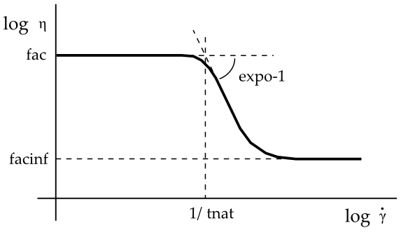
The Bird-Carreau law is commonly used when it is necessary to describe the low-shear-rate behavior of the viscosity. It differs from the Cross law primarily in the curvature of the viscosity curve in the vicinity of the transition between the plateau zone and the power law behavior.
The power law for viscosity is
 | (6–9) |
where  is the consistency factor,
  is the natural time, and
  is the power-law index, which is a property of a given
material.
is the power-law index, which is a property of a given
material.
The units for the parameters and their names in the Ansys Polymat interface are as follows:
| Parameter | Name in Ansys Polymat | Mass | Length | Time |
|---|---|---|---|---|

| fac | 1 | –1 | –1 |

| tnat | 1 | ||

| expo | – | – | – |
By default,  ,
,  , and
, and  are equal to 1. Figure 6.5: Power Law for Viscosity shows a plot of
  for the power law.
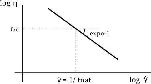
The power law is commonly used to describe the viscous behavior of polymeric materials, such as polyethylene, with shear rates greater than 2 or 3 decades. If the behavior at low shear rates must be fitted as well, the Bird-Carreau or Cross law will capture the plateau zone of the viscosity curve for low shear rates better than the power law.
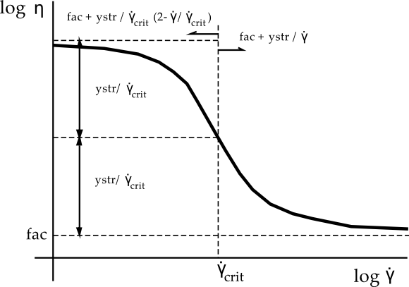
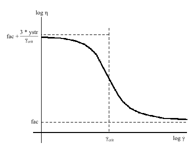
The Bingham law for viscosity is
 | (6–10) |
where  is the yield stress and
  is the critical shear rate, beyond which Bingham’s
constitutive equation is applied. For shear rates less than
is the critical shear rate, beyond which Bingham’s
constitutive equation is applied. For shear rates less than  , the behavior of the fluid is normalized in order to guarantee
appropriate continuity properties in the viscosity curve.
, the behavior of the fluid is normalized in order to guarantee
appropriate continuity properties in the viscosity curve.
The units for the parameters and their names in the Ansys Polymat interface are as follows:
| Parameter | Name in Ansys Polymat | Mass | Length | Time |
|---|---|---|---|---|

| fac | 1 | –1 | –1 |

| ystr | 1 | –1 | –2 |

| gcrit | – | – | –1 |
By default,  ,
,  , and
, and  are equal to 1. Figure 6.6: Bingham Law for Viscosity shows a plot of
  for the Bingham law.
The Bingham law is commonly used to describe materials such as concrete, mud, dough, and toothpaste, for which a constant viscosity after a critical shear stress is a reasonable assumption, typically at rather low shear rates.
A modified Bingham law for viscosity is also available:
 | (6–11) |
where  .
.
The units for the parameters and their names in the Ansys Polymat interface are as follows:
| Parameter | Name in Ansys Polymat | Mass | Length | Time |
|---|---|---|---|---|

| fac | 1 | –1 | –1 |

| ystr | 1 | –1 | –2 |

| gcrit | – | – | –1 |
By default,  ,
,  , and
, and  are equal to 1. Figure 6.7: Modified Bingham Law for Viscosity shows a plot
of
are equal to 1. Figure 6.7: Modified Bingham Law for Viscosity shows a plot
of  for the modified Bingham law.
Compared to the standard Bingham law, the modified Bingham law is an analytic
expression, which means that it may be easier for Ansys Polyflow to calculate,
leading to a more stable solution. The value  has been selected so that the standard and modified Bingham
laws exhibit the same behavior above the critical shear rate,
has been selected so that the standard and modified Bingham
laws exhibit the same behavior above the critical shear rate,  .
.
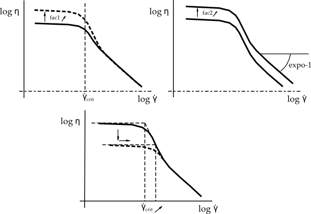
The Herschel-Bulkley law for viscosity is
 | (6–12) |
where  is the yield stress,
  is the critical shear rate,
  is the consistency factor, and
  is the power-law index.
The units for the parameters and their names in the Ansys Polymat interface are as follows:
| Parameter | Name in Ansys Polymat | Mass | Length | Time |
|---|---|---|---|---|

| fac1 | 1 | –1 | –2 |

| fac2 | 1 | –1 | –1 |

| gcrit | – | – | –1 |

| expo | – | – | –1 |
By default,  ,
,  ,
,  , and
, and  are equal to 1. Figure 6.8: Herschel-Bulkley Law for Viscosity shows a plot of
  for the Herschel-Bulkley law.
Like the Bingham law, the Herschel-Bulkley law is commonly used to describe materials such as concrete, mud, dough, and toothpaste, for which a constant viscosity after a critical shear stress is a reasonable assumption. In addition to the transition behavior between a flow and no-flow regime, the Herschel-Bulkley law exhibits a shear-thinning behavior that the Bingham law does not.
A modified Herschel-Bulkley law is also available:
 | (6–13) |
The units for the parameters and their names in the Ansys Polymat interface are as follows:
| Parameter | Name in Ansys Polymat | Mass | Length | Time |
|---|---|---|---|---|

| fac1 | 1 | –1 | –2 |

| fac2 | 1 | –1 | –1 |

| gcrit | – | – | –1 |

| expo | – | – | –1 |
By default,  ,
,  ,
,  , and
, and  are equal to 1. Figure 6.9: Modified Herschel-Bulkley Law for Viscosity shows a plot of
  for the modified Herschel-Bulkley law.

Compared to the standard Herschel-Bulkley law, the modified Herschel-Bulkley
law is an analytic expression, which means that it may be easier for
Ansys Polyflow to calculate, leading to a more stable solution. The integer value
3 that appears in the argument of the exponential term has been selected so that
the standard and modified Herschel-Bulkley laws exhibit the same behavior above
the critical shear rate,  .
.
The Cross law for viscosity is
 | (6–14) |
| where |

| = | zero-shear-rate viscosity |

| = | natural time (that is, inverse of the shear rate at which the fluid changes from Newtonian to power-law behavior) | |

| = | Cross-law index (=
1– for large shear rates) for large shear rates) |
The units for the parameters and their names in the Ansys Polymat interface are as follows:
| Parameter | Name in Ansys Polymat | Mass | Length | Time |
|---|---|---|---|---|

| fac | 1 | –1 | –2 |

| tnat | 1 | ||

| expom | – | – | – |
By default,  is equal to 1, and
  and
and  are equal to 0. Figure 6.10: Cross Law for Viscosity shows a plot of
  for the Cross law.
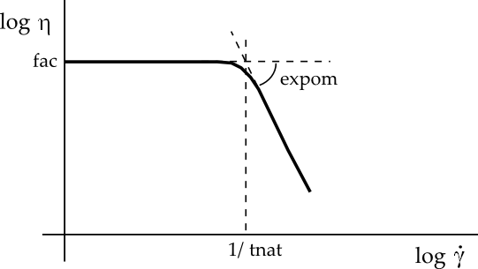
Like the Bird-Carreau law, the Cross law is commonly used when it is necessary to describe the low-shear-rate behavior of the viscosity. It differs from the Bird-Carreau law primarily in the curvature of the viscosity curve in the vicinity of the transition between the plateau zone and the power law behavior.
A modified Cross law for viscosity is also available:
 | (6–15) |
The units for the parameters and their names in the Ansys Polymat interface are as follows:
| Parameter | Name in Ansys Polymat | Mass | Length | Time |
|---|---|---|---|---|

| fac | 1 | –1 | –2 |

| tnat | 1 | ||

| expom | – | – | – |
By default,  is equal to 1, and
  and
and  are equal to 0. Figure 6.11: Modified Cross Law for Viscosity shows a plot of
  for the Cross law.
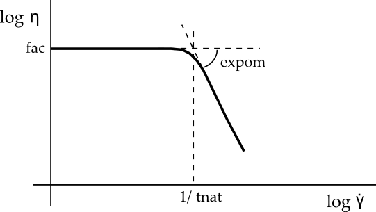
This law can be considered a special case of the Carreau-Yasuda viscosity law
(Equation 6–17),
where the exponent  has a value of 1.
The log-log law for viscosity is
 | (6–16) |
where  is the zero-shear-rate viscosity and
  ,
,  , and
, and  are the coefficients of the polynomial expression.
The units for the parameters and their names in the Ansys Polymat interface are as follows:
| Parameter | Name in Ansys Polymat | Mass | Length | Time |
|---|---|---|---|---|

| a0 | – | – | – |

| a1 | – | – | – |

| a11 | – | – | – |

| fac | 1 | –1 | –1 |

| gcrit | – | – | –1 |
By default,  and
and  are equal to 1, and
  ,
,  , and
, and  are equal to 0. Figure 6.12: Log-Log Law for Viscosity shows a plot of
  for the log-log law.
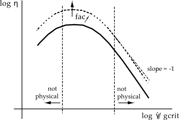
This viscosity law is purely empirical, but sometimes provides a better fit to experimental data than the others. Nevertheless, you should pay special attention to the coefficients you specify for the log-log law, as detailed below.
The function is a parabola in the ( ) space. Depending on the values of the polynomial
coefficients, the viscosity may decrease as the shear rate approaches zero,
which does not reflect physical behavior. Moreover, for high shear rates, the
slope of the curve may be less than –1, which is also not physical. When
you are using the log-log law, you must therefore ensure that the range of shear
rates in your application lies within the range of physically acceptable shear
rates for the law. This is accomplished by careful specification of the
polynomial coefficients.
) space. Depending on the values of the polynomial
coefficients, the viscosity may decrease as the shear rate approaches zero,
which does not reflect physical behavior. Moreover, for high shear rates, the
slope of the curve may be less than –1, which is also not physical. When
you are using the log-log law, you must therefore ensure that the range of shear
rates in your application lies within the range of physically acceptable shear
rates for the law. This is accomplished by careful specification of the
polynomial coefficients.
Important: Note that, for non-isothermal flows using the log-log law, the mixed-dependence law (described in Mixed-Dependence Law) must be used for the thermal dependence of the viscosity.
The Carreau-Yasuda law for viscosity is
 | (6–17) |
| where |

| = | zero-shear-rate viscosity |

| = | infinite-shear-rate viscosity | |

| = | natural time (that is, inverse of the shear rate at which the fluid changes from Newtonian to power-law behavior) | |

| = | index that controls the transition from the Newtonian plateau to the power-law region | |

| = | power-law index |
The units for the parameters and their names in the Ansys Polymat interface are as follows:
| Parameter | Name in Ansys Polymat | Mass | Length | Time |
|---|---|---|---|---|

| fac | 1 | –1 | –1 |

| facinf | 1 | –1 | –1 |

| tnat | 1 | ||

| expo | – | – | – |

| expoa | – | – | – |
By default,  ,
,  , and
, and  are equal to 1, and
  and
and  are equal to 0. Figure 6.13: Carreau-Yasuda Law for Viscosity shows a
plot of
are equal to 0. Figure 6.13: Carreau-Yasuda Law for Viscosity shows a
plot of  for the Carreau-Yasuda law.
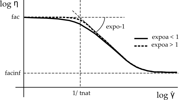
The Carreau-Yasuda law is a slight variation on the Bird-Carreau law (Equation 6–8). The addition
of the exponent  allows for control of the transition from the Newtonian
plateau to the power-law region. A low value (
allows for control of the transition from the Newtonian
plateau to the power-law region. A low value ( < 1) lengthens the transition, and a high value
(
< 1) lengthens the transition, and a high value
( >1) results in an abrupt transition.