


This section demonstrates how to use Ansys Polymat to perform automatic fitting. You will read in the experimental data from the curve file saved at the end of the non-automatic procedure.
Start a new session of Ansys Polymat by typing
polymat, as described in Starting Ansys Polymat. The first step is
to define the type of fluid model you want. Click the Select Fluid
Model menu item in the Ansys Polymat menu.
![]() Select Fluid Model
Select Fluid Model
The default selection is for an isothermal Generalized Newtonian model, so you can simply select Upper level menu to return to the main menu.
Now you can choose the power-law model and fix values for any parameters that you do not want to be involved in the fitting calculation. In the Ansys Polymat menu, click Material Data.
![]() Material Data
Material Data
Then click Shear-rate dependence of viscosity.
![]() Shear-rate dependence of viscosity
Shear-rate dependence of viscosity
In the resulting menu, click Power law.
![]() Power law
Power law
By default, all parameters (K, λ, and n) are subject to modification during the fitting calculation. Since you are interested in fitting the curve for the case where λ=1, you can fix the value of λ so that it remains constant during the fitting calculation.
To fix the value of λ, first click the menu button. Click when Ansys Polymat informs you that fixing is enabled. Click Modify tnat and click to keep the default value of 1.
![]() Modify tnat
Modify tnat
Then click tnat is a fixed value to specify that λ is to remain constant during the fitting calculation.
![]() tnat is a fixed value
tnat is a fixed value
Click Upper level menu, and then click the menu button again to disable fixing.
Click Upper level menu three more times to return to the top-level Ansys Polymat menu.
In the top-level Ansys Polymat menu, click Automatic fitting.
![]() Automatic fitting
Automatic fitting
Then click Add experimental curves.
![]() Add experimental curves
Add experimental curves
Click Add a new curve.
![]() Add a new curve
Add a new curve
Click Enter the name of the curve file and, in the resulting dialog box, select the file sample.crv you created previously and click .
![]() Enter the name of the curve file
Enter the name of the curve file
Click Upper level menu twice to return to the Automatic Fitting menu.
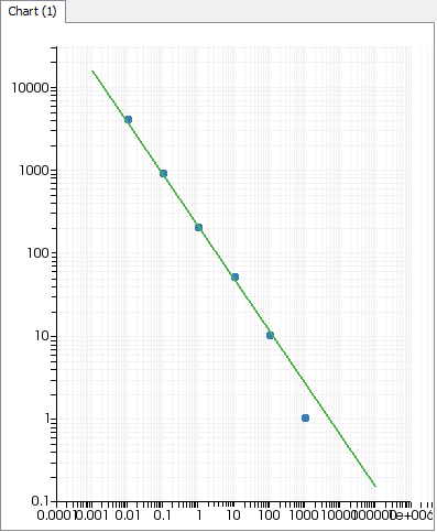
In the Automatic Fitting menu, click Draw experimental curves to plot the experimental data points in the chart.
![]() Draw experimental curves
Draw experimental curves
As discussed in the non-automatic procedure, the range of shear rates that is of interest is from 0.1 to 10. To limit the range for the fitting calculation, begin by clicking Numerical options for fitting in the Automatic Fitting menu.
![]() Numerical options for fitting
Numerical options for fitting
Then click Modify the window of shear rates and, when
prompted, enter 0.1 for the minimum shear rate and
10 for the maximum.
![]() Modify the window of shear rates
Modify the window of shear rates
Click Upper level menu to return to the Automatic Fitting menu.
Before you run the automatic fitting, you need to provide a name for the file where Ansys Polymat will save the results of the fitting calculation. You can read this material data file into Ansys Polydata when you are setting up the flow simulation, or read it into a later Ansys Polymat session to examine the curves again or perform further fitting.
To define the filename for the material data file, click Enter the name of the result file in the Automatic Fitting menu.
![]() Enter the name of the result file
Enter the name of the result file
Specify the name auto.mat in the Enter the
name of the mat file dialog box that opens, and click
.
Click the Run fitting... menu item in the Automatic Fitting menu.
![]() Run fitting...
Run fitting...
Ansys Polymat will automatically compute the shear viscosity curve, save the results to the auto.mat file, and update the chart to show the computed and experimental curves. Figure 1.9: Automatically Computed Viscosity Curve shows the resulting chart.
You can view calculated parameter values by clicking the View listing of fitting menu item in the Automatic fitting menu.
![]() View listing of fitting
View listing of fitting
The values of the parameters for this sample session are as follows: K=208.0, λ=1, and n=0.3723. These values are close to those you determined using the non-automatic procedure, but the automatic procedure has provided a slightly more accurate result with much less effort from you.
You can end the Ansys Polymat session by clicking Exit from the File drop-down menu, located at the top left side of the application window.
File → Exit