


This multi-part basic tutorial assumes that you have imported field and scalar data as described in Importing Field and Scalar Data and learned more about statistical analysis and result visualization in Analyzing Imported Field Data. You are now ready for:
In the DOE, 100 field designs have been calculated with a set of varying input parameters. A field-MOP is a reduced order model (ROM) for predicting the resulting field quantity for a new set of input parameters. During field-MOP creation, oSP3D calculates Field-CoP[Total] (Coefficient of Prognosis), indicating the model's forecast quality.
Note: To ensure that the Field-MOP is created, deactivate incomplete designs. Select > .
To create a field-MOP:
Select > > .
In the dialog box that opens, the Select training data tab is active by default.
Drag and drop the following quantity identifiers into the Input (selectable) area:
E_Modul
blank_thickness_1
plastic_failure
poisson_ratio
real_mat_abs_1
real_mat_ord_1
rho
yield_stress
Drag and drop the following quantity identifiers into the Output area:
pstrain
thickness
Because this example uses all default settings, no changes are necessary on the Settings tab.
Click .
Once oSP3D completes the calculations, it adds new result field quantities to the data table.
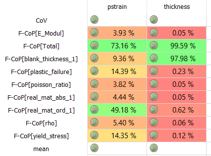
- F-CoP[Total]
The percentage value representing a variance-weighted average of the field model's forecast quality. Values above 80% are acceptable, and values above 90% are good. When the value for Field-CoP[Total] is low, the level of prediction might be good locally. However, you should carefully analyze the Field-CoP's distribution in space.
- F-CoP[
input parameter] The percentage value representing a variance-weighted average of the input parameter's explained variance of the resulting output field. Higher values indicate a higher sensitivity of the field model with respect to the input parameter.
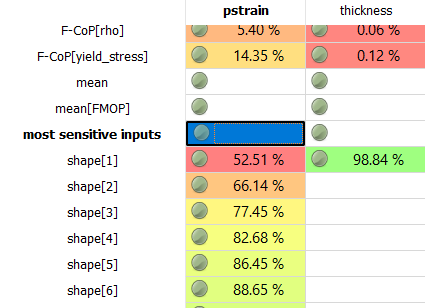
- most sensitive inputs
The most sensitive input parameter at each node or element on the mesh. If the value is unknown, the value for Field-CoP[Total] is too low to make a valid prediction. If the value is undefined, multiple inputs have exactly the same sensitivities.
- mean[FMOP]
The local average of the output field when varying the field model's input parameters.
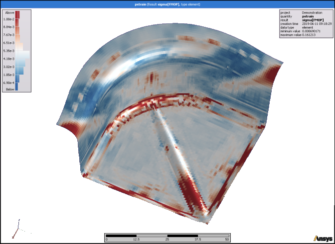
- sigma[FMOP]
The local standard deviation of the output field when varying the field model's input parameters.
You can now visualize the field-CoP results.
To visualize field-CoP results:
If the data table is not currently displayed, select > .
For the field quantity pstrain, select the most sensitive inputs result and press the Enter key to visualize.
The plot of the most sensitive inputs provides a good overview of the Field-MOP's behavior, allowing you to identify:
Areas of importance for each input parameter
Areas with low values for Field-CoP[Total], indicating little confidence in the field-MOP's ability to make a valid prediction
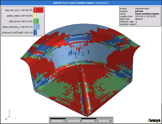
For example, if you select the result Field-CoP[Total] and press the Enter key, you can see the most sensitive inputs for the field quantity pstrain.
Select result field quantities from the data table and press the Enter key to visualize.
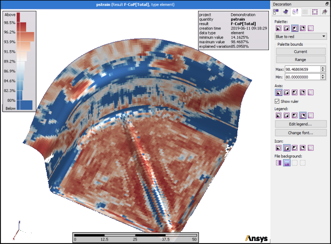
You can change the palette bounds in the visualization toolbox by clicking
 . In the
following plot for the result Field-CoP[Total], the minimum for
Field-CoP[Total] is set to 80%. The plot now clearly shows
significant local variations, depicting areas of acceptable
Field-CoP[Total].
. In the
following plot for the result Field-CoP[Total], the minimum for
Field-CoP[Total] is set to 80%. The plot now clearly shows
significant local variations, depicting areas of acceptable
Field-CoP[Total].
This next plot of the standard deviation of the field-MOP shows where the largest changes occur when the input parameters are varied. A good field-MOP has high values for F-CoP[Total] at the same points in space.
In this tutorial, Field-CoP[Total] shows significant local variation. Depending on the mesh areas of interest, the field model may be useable or require further refinement. The tutorial in Analyzing Imported Field Data, you excluded field designs with too many eroded elements, reducing the number of field designs from which to build the Field-MOP to 70. In cases like this, the preferred solution is to add more designs to the DOE and rebuild the Field-MOP from the larger dataset.
Note: While F-CoP values clearly identify one material parameter dominating the field model's output on average, the plot of most sensitive inputs tells a much more nuanced story, taking local variations into account.
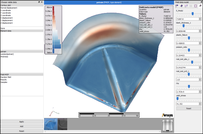
You can visualize a field-MOP's output field based on any input parameter set.
To visualize a field-MOP's output field based on any input parameter set:
In the Choose visible data window in the 3D visualization, select Element data, pstrain, and Field-MOP.
Click .
In the Field data model inspector, set the values for the input parameters by adjusting the sliders.
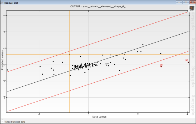
Field-MOPs can be analyzed with optiSLang postprocessing. Because outlier detection is a particularly useful feature, it is the focus in these topics:
Note: The file extension *.ombd must be associated with the optiSLang postprocessing executable (oslpp.exe)
To build a field-MOP with a MOP backend:
Select > .
Select > > .
In the dialog box that opens, the Select training data tab is active by default.
Drag and drop the desired quantity identifiers into the Input (selectable) area.
Drag and drop the quantity identifier pstrain into the Output area.
On the Settings tab, select Use MOP backend and accept the default MOP settings.
Click .
To indicate that existing field-MOPs can be overwritten, click .
Once oSP3D completes the calculations, you can open the field-MOP in optiSLang postprocessing.
To open a field-MOP in optiSLang postprocessing:
If the data table is not currently displayed, select > .
In the data table, select a field quantity with an existing field-MOP.
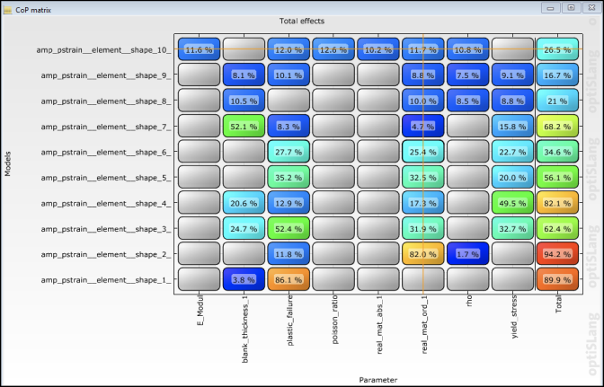
To generate a CoP matrix, select > > .
If prompted, select the optiSLang postprocessing app in which to open the file.
This CoP matrix shows that the first few random field amplitudes contribute the most to the field-MOP's variation. Any deviation from this pattern is an indication of model failure.
You can now detect outliers.
To deactivate outliers in oSP3D:
In the list of available objects, clear the check boxes for the respective field data objects.
Select > .
After deactivating the outliers, repeat all statistical analysis.
If desired, you can select > to save your data to your oSP3D database.