


This multi-part basic tutorial assumes that you have imported field and scalar data as described in Importing Field and Scalar Data and learned more about statistical analysis and result visualization as described in Analyzing Imported Field Data. You are now ready for:
In the DOE, 100 field designs have been calculated with a set of varying input parameters. An empirical random field model captures as much of the variation observed in the 100 field designs as possible with the smallest number of scalar random field amplitudes.
To create an empirical random field model:
Select > > .
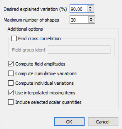
While this example has you accept the defaults shown, to get a more accurate random field model, you would increase the values for Desired explained variation (%) and Maximum number of shapes.
Random field decomposition is cut off when reaching the value specified for Maximum number of shapes, without achieving the desired explained variation percentage. In the worst case, if the field designs are entirely uncorrelated, 100 shapes are required to represent the 100 field designs with 100% accuracy.
Click to accept the defaults.
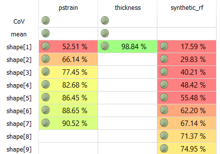
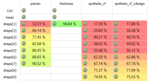
In the data table, oSP3D adds new data objects to the database:
oSP3D adds one field data object for each shape and the total explained variation.
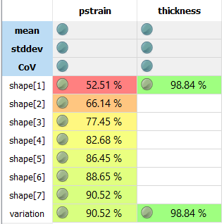
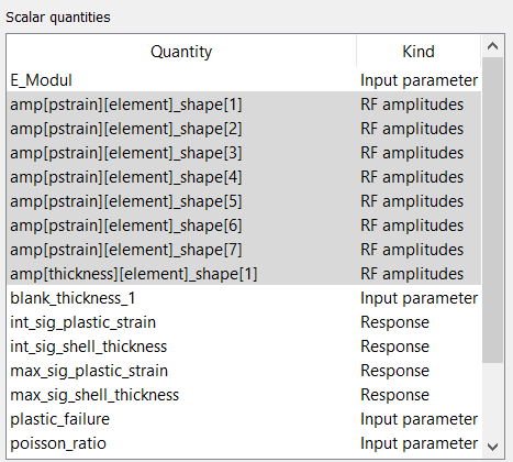
oSP3D adds a scalar quantity for each random field amplitude.
If the data table is not currently displayed, select > .
From the list of data objects, select shape[1] and variation and press the Enter key to visualize.
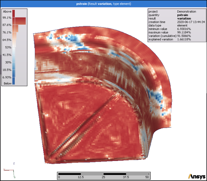
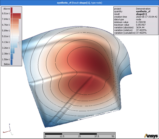
The following image shows a strongly localized effect. Of the variation observed in the field designs, approximately 55% is explained by the first shape of the empirical random field.
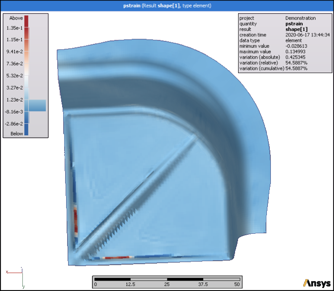
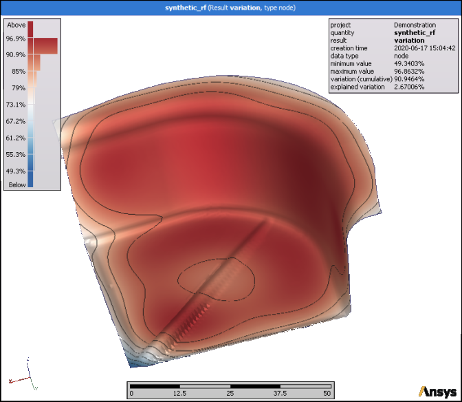
This next image shows the variation explained by the empirical random field. Comparing this plot to the variance plot of all field designs allows you to see that the explained variation is low only at locations where the variance is low. This is typical for empirical random fields and acceptable behavior.
The options for creating a synthetic random field model depends on whether field designs are available:
To create a synthetic random field model when no field designs are available:
If the data table is not currently displayed, select > .
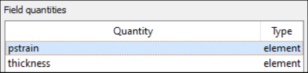
In the data table, select the field quantity pstrain.
Select > > .
In the dialog box that opens, for Ident, type
synthetic_rf: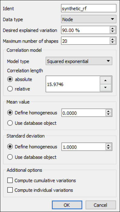
For Correlation length, select relative and then decrease the absolute value to 20.00 % to create a larger number of more localized shapes.
A relative correlation length of 20.00 % is a good starting value.
Click .
oSP3D adds one field data object for each shape and the total explained variation.
From the list of data objects, select the synthetic_rf values for shape[1] and variation and then press the Enter key to visualize.
The following image shows the general shape that is created when there is no prior knowledge from field designs.
This next image shows the variation explained by the synthetic random field declines near the edges of the structure.
To create a synthetic random field model when one to five field designs are available:
If the data table is not currently displayed, select > .
In the data table, select the field quantity pstrain.
Select > > .
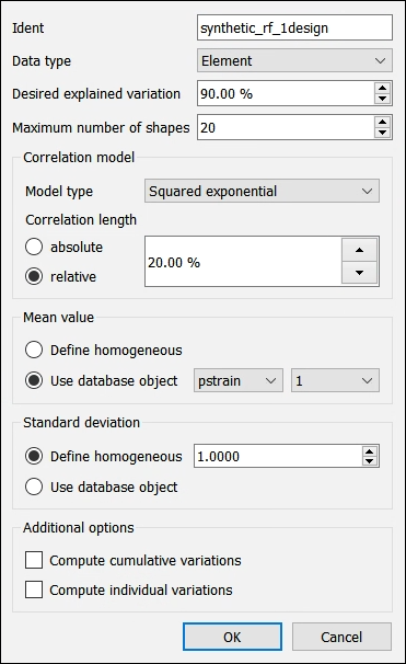
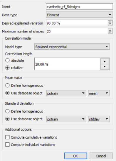
In the dialog box that opens:
For Ident, type
synthetic_rf_1design.For Data type, select Element.
For Correlation length, select relative and set the absolute value to 20.00 %.
For Mean value, select Use database object and select the first field design as if only one measurement or simulation was performed.
Note: If a small number of field designs is available, you can estimate the standard deviation and provide additional information to the synthetic random field model.
The dialog box should now look like this:
Click .
oSP3D adds one field data object for each shape and the total explained variation.
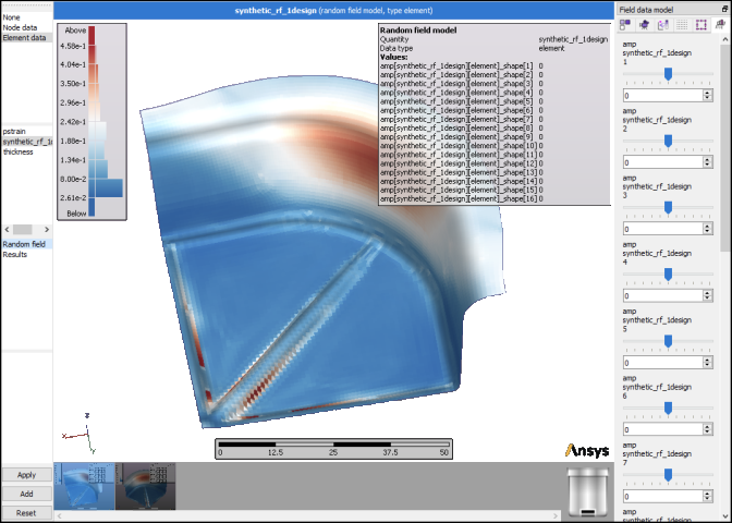
In the Choose visible data window for the 3D visualization, select Element data, synthetic_fr_1design, and Random field.
Click .
In the following image, the mean value for the synthetic random field is modeled after the single available field design. If you move the sliders, you can see that the shapes of the empirical random field are still general because no variation can be inferred from a single design.
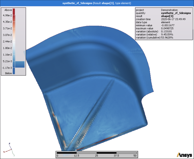
Assume that you created a synthetic random field with the mean and standard deviation estimated from five field designs:
This next image shows that with more field designs available to provide mean and standard deviation estimates, shapes reflecting the observed variation can be created.
If desired, you can select > to save your data to your oSP3D database.