


This multi-part basic tutorial assumes that you have imported field data defined on a unique mesh as described in Importing Field and Scalar Data and are now ready for:
Note: Statistical measures across multiple field designs are themselves fields. For example, the mean field indicates the average of all field designs at every point in space.
Designs with too many eroded elements can lead to questionable results. To exclude designs above a certain threshold from further analysis:
Select > .
Set Largest acceptable number of eroded data to 80 and click .
Verify the log message indicating the number of deactivated designs.
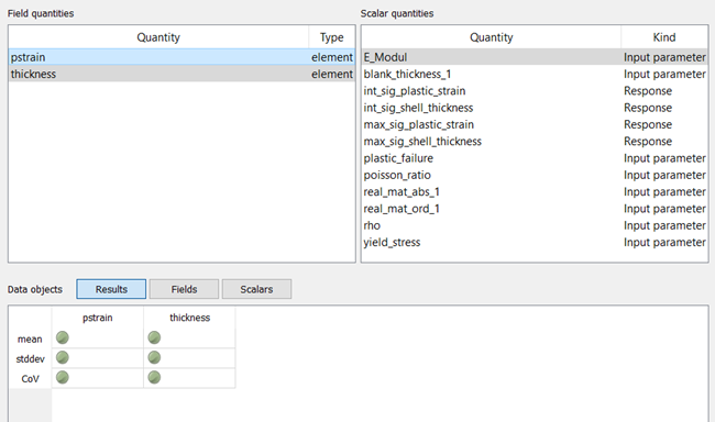
If the data table is not currently displayed, select > .
From the Data objects toggles, ensure the view is toggled on (button is blue) and the and views are off (buttons are gray).
In the list of individual scalar data objects, observe which check boxes are now cleared.
You are now ready to calculate standard statistical estimators.
Statistical measures are calculated using active samples only.
To calculate standard statistical estimators:
If the data table is not currently displayed, select > .
From the Field quanties list, select any number of field quantities for analysis.
For example, select both pstrain and thickness.
Select > > .
Select > > .
Select > > .
From the Data objects toggles, click the button to turn this view off (button is gray) and click the button to turn the view on (button is blue).
The data table now contains the resulting field data objects for the field quantities that you selected. The statistical measures are themselves fields. Every single mesh element in space is evaluated separately across all active field designs. This evaluation is valid because all field designs are defined on the unique reference mesh.
You can now visualize the resulting statistical measures.
To extract all information, visualize the resulting statistical measures:
From the list of data objects, select the resulting statistical measures and press the Enter key.
oSP3D adds stamps in the gray area of the visualization.
In the Manage views inspector, click the icon for showing two scenes at one time (
 ), splitting the scenes horizontally.
Drag a scene from the ribbon at the bottom into the Empty scene pane.
Rotate the view to your liking.
In the Manage views inspector, click .
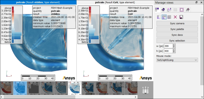
Differences in plastic strain between field designs are strongly localized in space. Any meaningful analysis of the reliability for the deep drawing process would be impossible from single-value measures alone. With this visualization of the resulting fields of statistical measures, identifying specific locations of interest to look at for optimizing the deep drawing process is straightforward.
You can now create and analyze random fields and field-MOPs. If desired, you can first select > to save your data to your oSP3D database.