Now that the mesh has been defined, you can set up the models and solver options using the guided tasks in the Simulate Workflow tree. In many cases, default parameters are assumed and employed, so that no input is required. The required inputs and changes (non-default) to the setup panels for this case are described here.
Note: You can change the display properties of items in the 3-D View by selecting them in the Workflow tree and right-clicking then selecting options from the context menu, such as turning ON/OFF their visibility or display of the mesh or level of opacity.
In the Workflow tree, expand Models. In the following steps you will turn ON (check-mark) several models and configure parameters for them in their Editor panels.
Models > Chemistry/Materials: Select Chemistry/Materials. On the Chemistry/Materials icon bar, click the New Import Chemistry
 icon. This opens a file browser where you can navigate to a chemistry set
file. For this project, however, we use a pre-installed chemistry set that comes with
Ansys Forte. This is a simplified, reduced n-heptane mechanism that can be
used to represent the diesel fuel under conventional diesel-engine combustion conditions. To
load this file, browse to the Data directory and
locate the pre-installed file named
Diesel_1comp_35sp.cks. The
Data directory can be accessed from the file browser
by clicking the data radio button in the upper right-hand subpanel of the
browser window. The chemistry file is a standard Ansys Chemkin chemistry-set file. (More
information about this chemistry set and the files referenced within it can be found in the
Appendix E: Fuel Chemistry Sets Included with Ansys Forte
in the Ansys Forte User's Guide
.)
icon. This opens a file browser where you can navigate to a chemistry set
file. For this project, however, we use a pre-installed chemistry set that comes with
Ansys Forte. This is a simplified, reduced n-heptane mechanism that can be
used to represent the diesel fuel under conventional diesel-engine combustion conditions. To
load this file, browse to the Data directory and
locate the pre-installed file named
Diesel_1comp_35sp.cks. The
Data directory can be accessed from the file browser
by clicking the data radio button in the upper right-hand subpanel of the
browser window. The chemistry file is a standard Ansys Chemkin chemistry-set file. (More
information about this chemistry set and the files referenced within it can be found in the
Appendix E: Fuel Chemistry Sets Included with Ansys Forte
in the Ansys Forte User's Guide
.)Note: You can respond Yes or No to the "View chemistry set information?" prompt. A Yes response displays the chemistry set file in a viewer.
Models > Transport: For this node, keep all the default settings.
Models > Spray Model: Since this is a direct-injection case, turn ON (check) Spray Model to display its icon (action) bar in the Editor panel.
For the basic Spray Properties, keep the default values: select Radius of Influence Model for the Droplet Collision Model and set 0.2 cm as the Radius of Influence. The Use Vaporization Model option should be ON (checked, its default value).
Create Injector: Click Spray Model in the Workflow tree. The icon bar provides two spray-injector options: Hollow Cone or Solid Cone. For the diesel injector, click the New Solid Cone Injector
 icon. In the dialog that opens, name the Solid Cone Injector as
"Injector 1". This opens another icon bar and Editor panel
for the new solid-cone spray model. In the Editor panel, configure the model parameters for
the solid-cone spray model.
icon. In the dialog that opens, name the Solid Cone Injector as
"Injector 1". This opens another icon bar and Editor panel
for the new solid-cone spray model. In the Editor panel, configure the model parameters for
the solid-cone spray model.Composition: Select Create new... in the Composition drop-down menu under Settings and click the Pencil
 icon to open the Fuel Mixture Editor. In the Fuel Mixture panel,
click the Add Species button and select nc7h16
(that is, n-heptane) as the Species,
n-Tetradecane as the Physical Properties and
1.0 as the Mass Fraction. (Note that you must
press ENTER after all the values are present in the table.)
icon to open the Fuel Mixture Editor. In the Fuel Mixture panel,
click the Add Species button and select nc7h16
(that is, n-heptane) as the Species,
n-Tetradecane as the Physical Properties and
1.0 as the Mass Fraction. (Note that you must
press ENTER after all the values are present in the table.)At the bottom of the panel, type a name for the fuel composition, such as n-heptane. Click Save and Close the window.
In the Injector 1 Editor panel, set Inflow Droplet Temperature = 368 K.
Under the Injection Type, change the Parcel Specification to Number of Parcels and set Injected Parcel Count = 30,000.
Set Spray Initialization to Discharge Coefficient and Angle, and Discharge Coefficient = 0.7, and Cone Angle = 15.0 degrees.
Keep default values for Droplet Size Distribution and, under the Solid Cone Breakup Model Settings, the KH Model Constants, RT Model Constants, and Use Gas-Jet Model.
Create a Nozzle: Click the New Nozzle
 icon on the Injector 1 icon bar and name the
nozzle "Nozzle 1". Nozzle 1 then appears in the Workflow
tree, and the Editor panel and icon bar transform to allow specification of the Nozzle
geometry and orientation. In the Editor panel, set the Reference Frame parameters to specify
the nozzle location and direction. Keep the default Global Origin and
use the following settings:
icon on the Injector 1 icon bar and name the
nozzle "Nozzle 1". Nozzle 1 then appears in the Workflow
tree, and the Editor panel and icon bar transform to allow specification of the Nozzle
geometry and orientation. In the Editor panel, set the Reference Frame parameters to specify
the nozzle location and direction. Keep the default Global Origin and
use the following settings:Location: Coord. System= Cylindrical, with R = 0.15 cm, Θ = 22.5 degrees, and A = 19.368 cm.
Spray Direction: Coord. System= Spherical, with θ = 104.0 degrees, and Φ = 22.5 degrees.
Click Apply. You can see the nozzle appear at the top of the geometry. (You may need to make the Geometry non-opaque by right-clicking Geometry and reducing Opacity or changing the color of the nozzle itself, by right-clicking in the Workflow tree on the left side, to make the nozzle easier to see in the interior.)
Create an Injection: In the Workflow tree, click Injector 1 again and click the New Injection
 icon on the Injector 1 icon bar and name the
injection Injection 1. The new Injection item appears in the Workflow
tree, and the Editor panel and the icon bar transform to allow specification of the
injection properties. In the Editor panel, select Crank Angle as the
Timing option and then expand the subpanel to specify the
Start of injection as –22.5 ATDC and
Duration of injection as 7.75, respectively. Set
the Total Injected Mass = 0.0535 g.
icon on the Injector 1 icon bar and name the
injection Injection 1. The new Injection item appears in the Workflow
tree, and the Editor panel and the icon bar transform to allow specification of the
injection properties. In the Editor panel, select Crank Angle as the
Timing option and then expand the subpanel to specify the
Start of injection as –22.5 ATDC and
Duration of injection as 7.75, respectively. Set
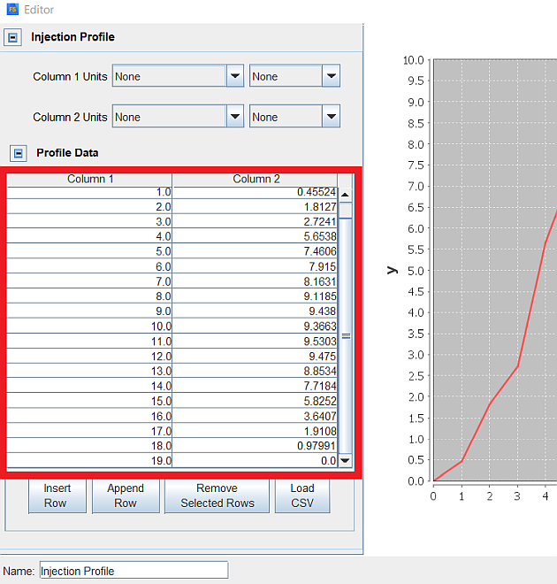
the Total Injected Mass = 0.0535 g.Injection Profile: Click the Create new... option in the profile selection menu next to Velocity Profile, then click the Pencil
icon to open a new window with the Profile Editor. In the Profile
Editor window, make sure all the Units are set to
None for both columns (the dimensionless data is automatically scaled
within Ansys Forte to match the mass and duration of injection) and click the Load
CSV button at the bottom of the panel (you may have to expand the panel size to
see the button). Navigate to the
InjectionProfile.csv
file (see Files for the Sample Diesel Sector Case
). Select
Comma as the Column delimiter and turn ON
Read Column Titles and load the profile file. Alternatively, you can
type in the Injection Profile data in the table on the Editor panel or copy and paste from a
spreadsheet or 3rd-party editor. Go to Profile Name at the bottom-left
of the panel and name the new profile Injection Profile. Once the data
is entered, click Save in the Profile Editor and then click
Apply in the Editor panel.
Models > Soot Model: Turn on the Soot Model. This creates the Settings item. In the Editor panel, do not change any of the defaults.
Boundary Conditions: Under Boundary Conditions in the Workflow tree, specify the boundary conditions in the Editor panels associated with each of the four boundary conditions created by importing the mesh. By default the Wall Model for all of the wall boundaries will be set to Law of the Wall. Leave this default setting as well as the default check box that turns ON heat transfer to the wall.
Boundary Conditions > Piston: Set Wall Temperature = 500.0 K. Turn ON Wall Motion with Motion Type set to Slider Crank. The other parameters should be:
For Reference Frame, accept the default Global Origin and Direction parameters.
Boundary Conditions > Periodicity: Accept the Sector Angle = 45 degrees, with multi-selected Periodic A and Periodic B boundaries on which to apply this boundary condition.
Note: Boundary conditions for sector-mesh cases cannot be modified. They are defined in the file that is imported to start the simulation. Automatic Mesh Generation cases have boundary conditions that can be modified.
Boundary Conditions > Head: Set Wall Temperature = 470.0 K. Click Apply.
Boundary Conditions > Liner: Set Wall Temperature = 420.0 K. Click Apply.
Initial Conditions > Region 1 Initialization (Main): Specify the parameters for the initial conditions as follows:
Composition: Select Constant and then Create new gas mixture... and click the Pencil
icon and to launch the Composition Editor. Set these parameters: set
the Composition = Mole Fraction (not the default Mass
Fraction). Then click the Add Species button and select both
o2 and n2 to add. When both
o2 and n2 are in the Species column in the
Composition table, enter 0.126 for the
o2 Fraction and 0.874 for n2.
Name this "Composition 1" in the text field at the bottom of the Gas Mixture
window. Click Save.Pressure: Select Constant and then 2.215 bar (Note: this is not the default unit.)
Turbulence: Select Constant and then in the pull-down menu for the Turbulence parameters, select Turbulent Kinetic Energy and Length Scale as the way in which we will specify the initial turbulence. For this option we provide an explicit value for the initial turbulent kinetic energy, but use a length-scale approximation to determine the turbulence intensity fraction. Use these values:
Velocity: Select Engine Swirl in the Velocity pull-down and then specify the swirl profile parameters:
Note: If you want to estimate the turbulence kinetic energy (TKE) as a fraction of the piston speed, let the fraction be F and stroke is ms-1, the value you would enter then would be

Under Piston Boundary, select Piston.
Simulation Controls: On the Editor panel, under Simulation Limits, for the Simulation End Point Option, specify:
Output Controls > Spatially Resolved: For the Spatially Resolved Output Control, specify:
Turn on Interval Based Crank Angle Outputs and set Output every to 5.0 degrees.
Also check the box next to User Defined Crank Angle Outputs and then create a table of data using the Profile Editor that contains crank angles going from -22 to +20, with increment 1, units of Angle Degree. Once the profile is saved and named UserCrankAngleOutputs, select it in the User-Defined Crank Angle drop-down menu. This assures that we get more resolved outputs around the spray, without requiring the same resolution throughout the simulation.
For Spatially Resolved Species, move these species to the Selection list: nc7h16, o2, n2, co2, h2o, co, no, and no2. Click Apply.
Output Controls > Restart Data: In the Workflow tree, check the box for Restart Data and then in the Restart panel, check the box that says, Write Restart File at Last Simulation Step. Uncheck any other boxes on the panel. Click Apply.
Preview Simulation > Boundary Motion. Accept the defaults and click the Play
 icon in the Boundary Motion icon bar. You will see the piston move up and
back down the cylinder through the interval defined in the Simulation Limits.
icon in the Boundary Motion icon bar. You will see the piston move up and
back down the cylinder through the interval defined in the Simulation Limits.Note: If the geometry elements are opaque, the piston is not visible. In this case, go to the Workflow tree on the left-hand side of the Simulate window and right-click Geometry and select Medium as the Opacity. Then make sure the Boundary Condition > Piston visibility
 is turned ON.
Save the project at this point using the File > Save command. Then continue to Running Your Quick Start Case [anchor> if you wish to run this case.