1.5.4. C) Create a 360° Mesh with the Automatic Mesh Generator (AMG)

Note: Running this simulation is estimated to take 2 hours 30 minutes on the Intel^® Xeon^® processor E5-2690 at 2.60 GHz (28 total cores).

The files for this tutorial are obtained by downloading the quick_start_360degree_automesh.zip file here .
Unzip quick_start_360degree_automesh.zip to your working folder.
To create a 360° mesh, start with an empty Simulate Interface and go to the Workflow tree and click Geometry. This opens the Geometry icon bar (Figure 1.6: Geometry icon bar ). On the Geometry icon bar, click the Import Geometry icon. In the resulting dialog, pull down and select Surfaces from one or more STL files. Navigate to the sample STL file (downloaded with the samples), Sandia_engine_geometry360.stl , and import it, accepting the default import options: mesh units of cm, accepting the default mesh units of cm and the data type as Unknown. When Unknown is selected, Ansys Forte will attempt to automatically determine the data type based on the contents of the file. If you cannot see the geometry after it loads, or to optimize the placement of the imported geometry, click the Refit icon on the toolbar (see Figure 1.16: Imported STL sample geometry with medium opacity in 3-D View panel ).
First, we verify that the geometry is watertight, which also means that the normals of each surface element must be pointed in the correct direction (outward, away from the fluid). If the geometry is not watertight, a message to that effect will be displayed in the Log window and a thick red line will be drawn along any edge where there is an "opening" between two surfaces. The Ansys Forte interface contains several mesh correction tools that can be used to address such issues. These are described in the User Guide. For this sample case, however, the mesh is already watertight. You can view the surface normals as follows:
1. Ansys Forte has a method to display the normal vectors. Right-click Geometry and turn ON Normals. Normals are indicated by small red lines that point away from the surface in the normal direction. For this case, you can verify that all surfaces have the normals directed outward.
  Figure 1.16: Imported STL sample geometry with medium opacity in 3-D View panel
Geometry:
1. Click the Geometry node in the Workflow tree. You should have only 3 surfaces: HEAD, LINER.2.2, and PISTON_BOWL.
2. You can right-click in the Workflow tree to set the opacity of all surfaces to Medium for the Geometry opacity. This sets the opacity of the surfaces associated with the Geometry node so you can see all of them. The surfaces still look "hairy" or "speckled" because the normals are displayed. If you want to turn OFF the normal, right-click in the Workflow tree and unselect Normals.
Mesh Controls:
1. Under Mesh Controls, we need to set the Material Point to a z location just below the cylinder head, to make sure it will always be "inside" the boundaries, and located at least one unit cell length away from any boundaries, when the piston is at TDC. To see the coordinate values for the head, select Geometry > head in the left-hand Workflow tree. The Editor panel below will show the min/max coordinates. From here we can see that the head is at z=17.52605 cm from the origin. The piston bowl has a depth of about 1 cm, so that you can set the material point about 0.5 cm below the head and be sure it will always be within the active boundaries. So, return to Mesh Controls > Material Point, and using the Reference Frame = Global Origin options, set z=17.0 cm and x=y=0 for the material point and click Apply. Once it is set, you can see it in the 3-D View panel (as a small cube) and it can be made visible/invisible in the by right-clicking in the Workflow tree on the left, under Mesh Controls.
2. In the Workflow tree, set the Global Mesh Size to 0.3 cm. This will set the default size of cells to be 3 mm long on each side of the cell cube. Click Apply.
  Note: For purposes of running a tutorial, a coarser Global Mesh Size of 0.3 cm allows the simulation to run faster. We suggest working with a global mesh size of 2–3 mm, depending on the size of the engine. For smaller-bore gasoline engines a smaller global mesh size is usually appropriate, while for larger-bore diesel or natural-gas engines, a larger global mesh size may be more appropriate.
3. Click the Mesh Controls node in the Workflow tree. In the icon bar, click the New Surface Refinement icon and name the new control AllSurfaces. (This indicates that along the selected surface, cells of this smaller size will be used.) A new surfaces item appears under Mesh Controls in the Workflow tree. In the panel that appears, select all three surfaces from the Location list, set the mesh Size as Fraction of Global Size to 1/2 with an extension of 1 layer. Click Apply.
4. Create another refinement control, a Solution Adaptive Mesh (SAM), based on velocity. Click the Mesh Controls node in the Workflow tree. In the icon bar, click the New Solution Adaptive Mesh icon on the Mesh Controls Editor panel. Name the new refinement control SAM-Velocity. In the SAM-Velocity Editor panel, set the Quantity Type = Gradient of Solution Field and Solution Variables = VelocityMagnitude. Set Bounds = Statistical and Sigma Threshold = 0.5. Set the Size as Fraction of Global Size = 1/4. The refinement is Active = During Crank Angle Interval, Start angle = –23 degrees and End angle = 50 degrees. The Location option is Entire Domain. Click Apply.
Models > Chemistry: Load the n-heptane ( Diesel_1comp_35sp.cks ) chemistry set (as described in Step 1 ).

Models > Spray Model:Turn on the Spray Model and set up the spray parameters. You will use the same steps as for the sector mesh example (Step 3 ), but this time you will first set up 1, then 8, nozzle holes (Nozzle 1, Nozzle 2, ... Nozzle 8), since you are no longer doing a 1/8th sector model.

Add an Injector (Solid-cone) as you did for the sector mesh, using the same (default) spray-model parameters. See Step 3 b .
Spray composition (same as for sector mesh). See Step 3 b .
Add the first Nozzle with same settings as for sector mesh, with Φ =22.5 degrees. See Step 3 c . Important: Change the Nozzle Height (A in the Cylindrical Location parameters) to 17.368 cm.
Add an Injection, with the same settings as for the sector mesh: SOI=‑22.5 CA, DOI=7.75 CA, total injected mass = 0.0535 g, and set up InjectionProfile using the imported CSV file, InjectionProfile.csv. Make sure that the units in the profile setup panel are set to None in both column 1 and in column 2. See Steps 3 d and 3 5 .

Now use the Copy and Paste icons on the icon bar to copy Nozzle 1 and repeatedly paste it to create Nozzle 2, Nozzle 3, ... Nozzle 8. For each one, shift the Location θ and Spray Direction Φ values by 45 degrees, so that you end up with a nozzle at 22.5, 67.5, 112.5, 157.5, 202.5, 247.5, 292.5, and 337.5 degrees. Verify the hole pattern from the spray cone visualizations shown in the 3-D View. You should have an evenly spaced pattern, as shown in Figure 1.17: Eight nozzles in sample engine .

Table 1.2: Settings for 8 nozzles in 360° case

Nozzle	Location θ	Spray Direction Φ
Nozzle 1 Set Height=17.368	22.5	22.5
Nozzle 2	67.5	67.5
Nozzle 3	112.5	112.5
Nozzle 4	157.5	157.5
Nozzle 5	202.5	202.5
Nozzle 6	247.5	247.5
Nozzle 7	292.5	292.5
Nozzle 8	337.5	337.5

Figure 1.17: Eight nozzles in sample engine

Boundary Conditions: In this step, we create 3 boundary conditions for walls and associate them with Liner, Head, and Piston, respectively.
1. Liner: From the Boundary Conditions node, click the New Wall icon and name it Liner. In the liner Editor panel, select the LINER.2.2 geometry item in the Location list. Select Law of the Wall, use Heat Transfer and set Wall Temperature to 420 K (as with the sector mesh). Click Apply.
2. Boundary Conditions > Head: Do the same, naming the Boundary Condition Head, but set the Wall Temperature to 470 K.
3. Boundary Conditions > Piston: Do the same, naming the Boundary Condition Piston, but set the Wall Temperature to 500 K. Here, for the piston, also check (turn ON) the Wall Motion option and select Slider Crank under the list of motion options. Then enter the engine parameters that control the crank motion: Stroke = 15.24 cm, Connecting Rod Length = 30.48 cm, Piston Offset = 0.0 cm. Keep the defaults for the Reference Frame and Movement Type.
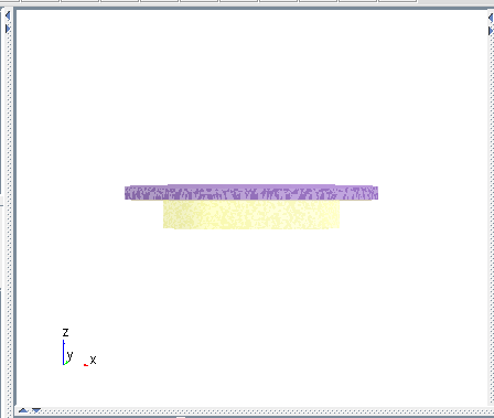
- With 3 boundaries defined, Liner, Head, and Piston, you can now right-click Geometry in the Workflow tree and Make None Visible for all the original geometry surfaces. Then you will just see the new boundary surfaces. Note that the Piston boundary gets translated automatically to its location at 0 CA by default, based on the slider-crank motion settings.
Initial Conditions > Default Initialization:
1. Set the default initialization in the same manner as for the sector mesh case (See Step 6 ): mole fractions (not mass) of o2, n2 = 0.126, 0.874, respectively; Temperature = 362.0, Pressure = 2.215 bar (note that this is not the default unit).
2. Set the parameters TKE = 92903.04 cm²/s² , Turbulence Length Scale = 1.12. These are equivalent to the initial values set as relative to piston speed in the sector-mesh specification.
3. Also select Velocity = Engine Swirl and set the swirl ratio parameters for initialization of the swirl flow relative to crank rotation:
  - Initial Swirl Ratio = 0.5
  - Initial Swirl Profile Factor = 3.11
  - Initialize Velocity Components Normal to Piston = ON
  - Under Piston Boundary, select Piston.
Simulation Controls > Simulation Limits: (This starts out the same as for the sector-mesh case, see Steps 7 and 8 ).
1. As with the sector mesh case, set the crank-angle limits from -165 to 125 CA, and set RPM = 1200 rpm and Cycle Type = 4-Stroke
2. Do not set a restriction on total time steps.
Simulation Controls > Time Step: Change the Initial Simulation Time Step to be 5.E-7 sec. The undistorted nature of the Cartesian mesh used in the automatic mesh generation allows for a larger time step to be used and this will speed the simulation.
Simulation Controls > Chemistry Solver: Repeat the settings from the sector mesh case (that is, use Dynamic Cell Clustering, Activate Chemistry as Conditionally, turn on After Fuel Injection Starts and When Temperature is Reached, with Threshold Temperature set to 600 K).
Output Controls > Spatially Resolved: For the Spatially Resolved Output Control, specify:
- Output Timing Control as Crank Angle
- Turn on Interval Based Crank Angle Outputs and set Output every = 10.0 degrees
- Also check the box next to User Defined Crank Angle Outputs and then create a table of data using the Profile Editor that contains crank angles going from -22 to +20, with increment 1, units of Angle and Degree. Once the profile is created and named UserCrankAngleOutputs, select it in the User-Defined Crank Angle Output. This assures that we get more resolved outputs around the spray, without requiring that resolution throughout the simulation.
- For Spatially Resolved Species, move these species to the Selection list: nc7h16, o2, n2, co2, h2o, co, oh, h2o2, no2, c2h2, c3h6, and soot. Click Apply.
Output Controls > Spatially Averaged And Spray:
- For the Spatially Averaged Output Control, select the Crank Angle option and specify Output Every = 1.0 degree.
- For Spatially Averaged Species, select all and move all species to the Selection list. Click Apply.
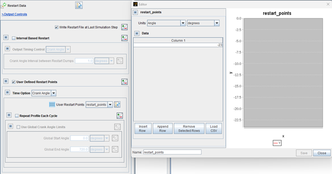
Output Controls > Restart Data: Check the box for Restart Data and then in the Restart panel, check the User Defined Restart Points option and select Create new... for User Restart Points. Open the profile editor and enter -23 degree ATDC (just before SOI). Uncheck any other boxes on the panel. Click Apply.
Figure 1.18: Restart Data Parameter Settings
Preview Simulation > Boundary Motion. Accept the defaults and click the Play icon in the Boundary Motion icon bar. You will see the piston move up and back down the cylinder through the interval defined in the Simulation Limits.
Preview Simulation > Mesh Generation: On the Mesh Generation Editor panel, set Time Option to Crank Angle and set the value to 0 CA degrees. This allows you to look at TDC and make sure you have enough cells in the squish region. Enter the Data Set Name as PreviewData. Click the Generate Mesh icon to view and export the mesh to Ansys EnSight.