


Once you are in the Fluent Remote Visualization Client you can display mesh, contours and vectors, modify solution settings (as long as the server is not calculating), start, pause, and interrupt calculations, and send commands.
From within a connected remote client session you can connect to up to 5 other servers (a single remote client can be connected to a maximum of 6 servers).
Click in the Actions ribbon tab (Connections group box).
 Actions → Connection
→ New Connection...
Actions → Connection
→ New Connection...This creates a new branch in the tree for the new remote session connection.
Connect to the new server—two scenarios:
Connect to an already-running Fluent server
Select the newly created sub-branch in the tree.
Click in the Server Info Filename field (highlighted in yellow in the Properties window), then click .
Select the server information file and click .
Connect to the server session by clicking Connect in the Actions ribbon tab (Connection group box).
Actions
→ Connection →
Connect
New server on the same machine as the client
Right-click the new sub-branch in the tree and select Start Server.
Specify the appropriate settings in the Fluent Launcher and click to launch Ansys Fluent. The new Fluent session is automatically connected to the client.
Use the help menu (![]() ) icon in the upper right-hand corner of the workspace to access its
documentation. Some workspaces even have field-level user assistance that provide
information and guidance about a particular field.
) icon in the upper right-hand corner of the workspace to access its
documentation. Some workspaces even have field-level user assistance that provide
information and guidance about a particular field.
In addition to Online Technical Resources..., and the Product Improvement Program, you can also obtain information about the version and release of Fluent you are running by selecting the Version... option in help menu.
You can specify global settings that are applied whenever you are operating in the Remote Visualization Client. These settings are case-independent and are controlled using the Preferences dialog box.
![]() File → Preferences...
File → Preferences...
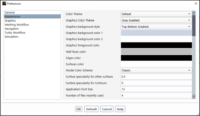
Note that there is only one Preferences file that applies to all Fluent workspaces. Not all preference settings are relevant to all workspaces. Refer to Setting User Preferences/Options in the Fluent User's Guide for additional information.
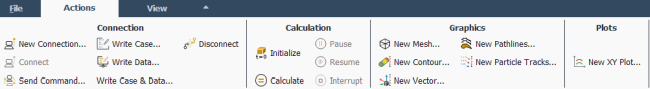
You have the ability to initialize, start, pause, and interrupt a calculation from the Remote Visualization Client. The buttons for these actions are located in the Actions ribbon tab.
—fills the flow field with an initial "guess" for the solution.
—begins the process of Fluent calculating the solution.
As soon as Fluent begins calculating, a progress monitor appears that visually indicates solution progress and the remaining number of time steps/iterations.
—"pauses" the calculation at the end of the iteration and waits for your input. When you click , Fluent continues calculating from where it was paused.
For example, if you request 10 iterations and pause at the 4th iteration, when you click , Fluent will calculate for the remaining 6 iterations.
If you are running from a script/journal file, Pause just "pauses" the run and all remaining commands will be executed when you click Resume.
Note: Do not switch from steady-state to transient (or vice versa) or change models when the calculation is paused.
—continues Fluent calculating the solution from the point where it was paused.
—stops the calculation and takes the solver out of the iteration loop. You must then click after adjusting the remaining iterations/time-steps.
For example, if you request 10 iterations and interrupt at the 4th iteration, when you click , Fluent will calculate for 10 additional iterations (14 iterations total).
If you are running from a script/journal file, Interrupt will cancel the run and the remaining commands will not be executed.
Select the Run Calculation branch in the tree to modify the Properties - RemoteSessionX: Run Calculation.

Important: Do not start calculations from the Send Command to Server dialog box—they must be started using the GUI on the client.
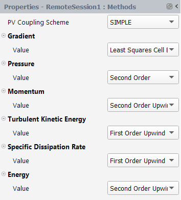
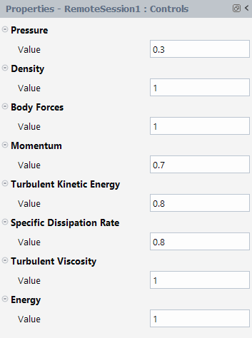
When calculations are stopped or paused, you can modify solution methods, solution controls, and convergence criteria from the Remote Visualization Client.
To modify the solution methods or controls:
Select Methods or Controls in the tree. This opens the Properties - Remote SessionX: Methods or Properties - Remote SessionX: Controls.
Modify the solution methods and controls as required. Modified settings are automatically synched with the server.
To modify convergence conditions:
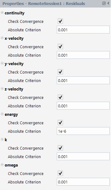
Select Residuals in the tree. This opens the Properties - Remote SessionX: Residuals or Properties - Remote SessionX: Controls.
Modify the convergence conditions as required. Modified settings are automatically synched with the server.
Note: If you want to enable or disable the plotting of residuals, you must do so from within the server session. Sending TUI commands to enable or disable residual plotting using the Send Command to Server dialog box only controls the status of residual plotting in the server, not in the Fluent Remote Visualization Client.
The graphics window lets you interact with and visualize your model. You can use the toolbars (Toolbars in the Fluent User's Guide) to manipulate the model view and you can use right-click context menus to create graphics objects, as shown in Figure 1.9: Creating a Contour Via the Context Menu. Refer to Graphics Objects for additional information on creating graphics objects.
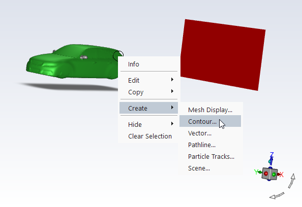
Context menus allow you to:
Print information about the selected surface(s) to the console.
Edit the currently displayed graphics object(s).
Copy the currently displayed graphics object(s).
Create new graphics objects.
Hide surfaces in the current display.
You can create different types of surfaces to visualize your results, including points, lines, rakes, planes, and iso-surfaces. Values are interpolated to the smoothed out boundary lines.
Refer to the following sections for more details:
You may be interested in displaying results at a single point in the domain. For example, you may want to monitor the value of some variable or function at a particular location. To do this, you must first create a "point" surface, which consists of a single point. When you display node-value data on a point surface, the value displayed is a linear average of the neighboring node values. If you display cell-value data, the value at the cell in which the point lies is displayed.
![]() Results → Surfaces
Results → Surfaces
![]() New → Point
New → Point
To create a point surface, use the Figure 1.10: Properties of a Point Surface.
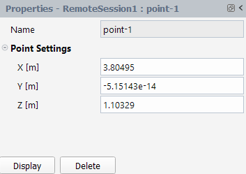
(Optional) Provide a name for the point surface if you do not want to use the default name.
Important: The surface name that you provide must begin with an alphabetical letter. If the name of the surface begins with any other character or number, Fluent rejects the entry.
Note: The Fluent Name field indicates the name of a surface within the Fluent workspace.
When a surface is created in the standard Fluent workspace, the Name field will match the Fluent Name field.
Surfaces created in the Remote Visualization Client may end up with a different name in the Fluent workspace. In this case, refer to the Fluent Name field to see a surface's name in the Fluent workspace.
Specify the location of the point. There are two different ways to do this:
Enter the coordinates (x, y, z) under Point Settings.
Move the point tool (
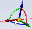 ) to the location in the domain where you want the point
surface created. Refer to Using the Point Tool in the Fluent User's Guide for additional
information.
) to the location in the domain where you want the point
surface created. Refer to Using the Point Tool in the Fluent User's Guide for additional
information.
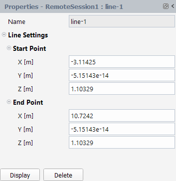
A line is simply a line that extends up to and includes the specified endpoints; data points will be located where the line intersects the faces of the cell, and consequently may not be equally spaced.
![]() Results → Surfaces
Results → Surfaces
![]() New → Line
New → Line
To create a line surface, use the Figure 1.11: Properties of a Line Surface.
(Optional) Provide a name for the line surface if you do not want to use the default name.
Important: The surface name that you provide must begin with an alphabetical letter. If the name of the surface begins with any other character or number, Fluent rejects the entry.
Note: The Fluent Name field indicates the name of a surface within the Fluent workspace.
When a surface is created in the standard Fluent workspace, the Name field will match the Fluent Name field.
Surfaces created in the Remote Visualization Client may end up with a different name in the Fluent workspace. In this case, refer to the Fluent Name field to see a surface's name in the Fluent workspace.
Specify the location of the Start Point.
Specify the location of the End Point.
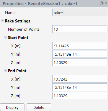
A rake consists of a specified number of points equally spaced between two specified endpoints.
![]() Results → Surfaces
Results → Surfaces
![]() New → Rake
New → Rake
To create a rake surface, use the Figure 1.12: Properties of a Rake Surface.
(Optional) Provide a name for the rake surface if you do not want to use the default name.
Important: The surface name that you provide must begin with an alphabetical letter. If the name of the surface begins with any other character or number, Fluent rejects the entry.
Note: The Fluent Name field indicates the name of a surface within the Fluent workspace.
When a surface is created in the standard Fluent workspace, the Name field will match the Fluent Name field.
Surfaces created in the Remote Visualization Client may end up with a different name in the Fluent workspace. In this case, refer to the Fluent Name field to see a surface's name in the Fluent workspace.
Set the Number of Points to include in the rake surface.
Specify the location of the Start Point.
Specify the location of the End Point.
To display flow-field data on a specific plane in the domain, you will use a plane surface. You can create surfaces that cut through the solution domain along arbitrary planes (3D cases only).
There are three types of plane surfaces that you can create:
Coordinate system-based—the plane is created in the YX, ZX, or XY directions, bounded by the extents of the domain. You can move the plane to the desired location in the domain using the plane tool. For example, if you are using the YZ Plane method, you can drag the plane in the (+) or (-) X direction.
Point and normal—the plane orientation is determined by selecting a point and specifying a direction normal to that point. The extents of the plane are the edges of the domain. You have the option to control the orientation of the plane using the plane tool or you can compute the normal from a surface.
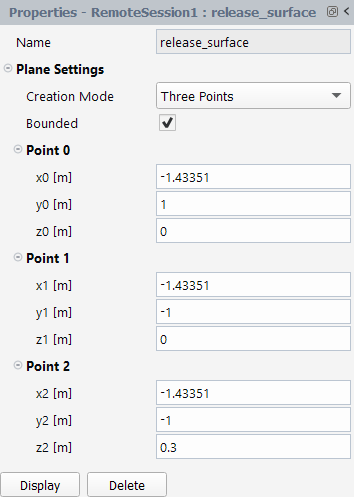
Three points—the plane orientation and extents are bounded by three points that you can select. You also have the option to manipulate the points and orientation of the plane directly in the graphics window using the plane tool.
![]() Results → Surfaces
Results → Surfaces
![]() New → Plane
New → Plane
To create a plane surface, use the Figure 1.13: Properties of a Plane Surface.
The procedure for creating the plane surface varies depending on the method you want to use.
Point and Normal
(Optional) Provide a name for the plane.
Important: The surface name that you enter must begin with an alphabetical letter. If the name of the surface begins with any other character or number, Fluent rejects the entry.
Note: The Fluent Name field indicates the name of a surface within the Fluent workspace.
When a surface is created in the standard Fluent workspace, the Name field will match the Fluent Name field.
Surfaces created in the Remote Visualization Client may end up with a different name in the Fluent workspace. In this case, refer to the Fluent Name field to see a surface's name in the Fluent workspace.
Drag the plane tool to the desired location, as shown in The Plane Tool for the Point and Normal Method in the Fluent User's Guide.
Alternatively, you can specify Point 0 and the Normal by providing the coordinates of each.
Bounded
(Optional) Provide a name for the plane.
Important: The surface name that you enter must begin with an alphabetical letter. If the name of the surface begins with any other character or number, Fluent rejects the entry.
Note: The Fluent Name field indicates the name of a surface within the Fluent workspace.
When a surface is created in the standard Fluent workspace, the Name field will match the Fluent Name field.
Surfaces created in the Remote Visualization Client may end up with a different name in the Fluent workspace. In this case, refer to the Fluent Name field to see a surface's name in the Fluent workspace.
Drag the plane tool to the desired location, as shown in The Plane Tool for the Three Points Method in the Fluent User's Guide.
Alternatively, you can specify Point 0, Point 1, and Point 2 by providing the coordinates.
Three Points
(Optional) Provide a name for the plane.
Important: The surface name that you enter must begin with an alphabetical letter. If the name of the surface begins with any other character or number, Fluent rejects the entry.
Note: The Fluent Name field indicates the name of a surface within the Fluent workspace.
When a surface is created in the standard Fluent workspace, the Name field will match the Fluent Name field.
Surfaces created in the Remote Visualization Client may end up with a different name in the Fluent workspace. In this case, refer to the Fluent Name field to see a surface's name in the Fluent workspace.
Drag the plane tool to the desired location, as shown in The Plane Tool for the Three Points Method in the Fluent User's Guide.
Alternatively, you can specify Point 0, Point 1, and Point 2 by providing the coordinates.
Multiple Planes
Instead of creating plane surfaces one at a time as described above, you have the option to create multiple plane surfaces at once using the Figure 1.14: Create Multiple Planes Dialog Box.
![]() Results → Surfaces
Results → Surfaces
![]() Create Multiple Planes...
Create Multiple Planes...
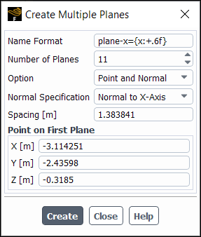
To use the Create Multiple Planes dialog box:
(Optional) Provide a format for naming the plane surfaces in the Name Format field.
Specify how many planes will be created in the Number of Planes field.
Select the method for how you want to create the planes in the Option drop-down list.
Point and Normal—similarly to the process described earlier in this section, you must provide a point and the direction normal to that point to define the first plane.
First and Last Point—you define the coordinates for the first and last point, which determines the orientation of the planes. The spacing is determined by how many planes you specify in the Number of Planes field.
(Point and Normal only) Specify the direction normal (perpendicular) to the plane in the Normal Specification drop-down list.
(Point and Normal only) Specify how far apart the planes are from each other in the Spacing field.
Provide the coordinate for the location of the first plane in the Point on First Plane group box.
(First and Last Point only) Provide the coordinates for the location of the last plane in the Point on Last Plane group box.
Click to create the new plane surfaces.
The new plane surfaces created using the Create Multiple Planes dialog box are added to the Outline View tree under the Surfaces branch and are now eligible for editing individually. Once created, the multiple planes cannot be edited as a group.
If you want to If you want to display results on cells that have a constant value for
a specified variable, you will need to create an iso-surface of that variable. Generating
an iso-surface based on  ,
,  , or
, or  coordinate, for example, will give you an
  ,
,  , or
, or  cross-section of your domain; generating an iso-surface based on
pressure will enable you to display data for another variable on a surface of constant
pressure. You can create an iso-surface from an existing surface or from the entire
domain. Furthermore, you can restrict any iso-surface to a specified cell zone.
cross-section of your domain; generating an iso-surface based on
pressure will enable you to display data for another variable on a surface of constant
pressure. You can create an iso-surface from an existing surface or from the entire
domain. Furthermore, you can restrict any iso-surface to a specified cell zone.
Important: Note that you cannot create an iso-surface until you have initialized the solution, performed calculations, or read a data file.
![]() Results → Surfaces
Results → Surfaces
![]() New → Iso-Surface
New → Iso-Surface
To create an iso-surface, use the Figure 1.15: Properties of an Iso-Surface.
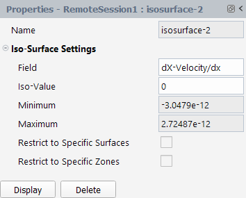
(Optional) Provide a name for the iso-surface.
Important: The surface name that you enter must begin with an alphabetical letter. If the name of the surface begins with any other character or number, Fluent rejects the entry.
Note: The Fluent Name field indicates the name of a surface within the Fluent workspace.
When a surface is created in the standard Fluent workspace, the Name field will match the Fluent Name field.
Surfaces created in the Remote Visualization Client may end up with a different name in the Fluent workspace. In this case, refer to the Fluent Name field to see a surface's name in the Fluent workspace.
Click Field to open the Field dialog box and specify the field you want to view.
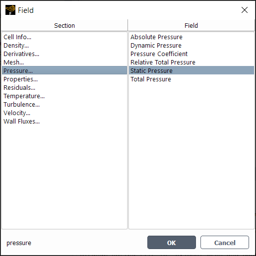
Click to confirm your selected field and close the dialog box.
Enter the iso-values into the Iso-Value field. You can enter multiple iso-values into the field separated by spaces.
Set the range by specifying the Minimum and Maximum.
(Optional) Enable Restrict to Specific Surface to only display iso-values on specific surfaces. Click in the yellow Surfaces list that appears, select the desired surfaces and click to confirm the selection and close the dialog box.
(Optional) Enable Restrict to Specific Cell Zones to only display iso-values on specific zones. Click in the yellow Zones list that appears, select the desired zones and click to confirm the selection and close the dialog box.
Click at the bottom of the iso-surface properties to delete an iso-surface.
Instead of creating iso-surfaces one at a time as described above, you have the option to create multiple iso-surfaces at once using the Figure 1.16: Create Multiple Iso-Surfaces Dialog Box.
Create Multiple Iso-Surfaces
Instead of iso-surfaces one at a time as described above, you have the option to create multiple iso-surfaces at once using the Figure 1.16: Create Multiple Iso-Surfaces Dialog Box.
![]() Results → Surfaces
Results → Surfaces
![]() Create Multiple Iso-Surfaces...
Create Multiple Iso-Surfaces...
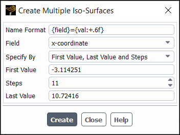
To use the Create Multiple Isosurfaces dialog box:
(Optional) Provide a format for naming the iso-surfaces in the Name Format field.
Select the field that you want to use for creating the iso-surfaces from the Field drop-down list:
rmse-y-velocity—root mean square error of the y-component of the velocity.
rmse-x-velocity—root mean square error of the x-component of the velocity.
rmse-pressure—root mean square error of gauge pressure.
mean-y-velocity—average of the y-component of the velocity.
mean-velocity-magnitude—average of the velocity magnitude.
mean-pressure—average gauge pressure.
y-coordinate—value of the y-coordinate.
mean-z-velocity—average of the z-component of the velocity.
total-pressure—value of the total gauge pressure.
z-coordinate—value of the z-coordinate.
axial-coordinate—value of the axial-coordinate.
rmse-z-velocity—root mean square error of the z-component of the velocity.
y-vorticity—y-component of the vorticity.
z-velocity—z-component of the velocity.
velocity-magnitude—magnitude of the velocity.
x-coordinate—value of the x-coordinate.
z-vorticity—z-component of the vorticity.
helicity—the combination of spin and velocity of the flow.
vorticity-mag—magnitude of the vorticity.
cell-volume—value of the mesh cell volume.
viscosity-lam—laminar viscosity.
x-velocity—x-component of the velocity.
y-velocity—y-component of the velocity.
mean-x-velocity—average of the x-component of the velocity.
dynamic-pressure—value of the dynamic pressure.
x-vorticity—x-component of the vorticity.
angular-coordinate—value of the angular coordinate.
absolute-pressure—value of the absolute pressure.
pressure—value of the pressure.
rmse-velocity-magnitude—root mean square error of the velocity magnitude.
abs-angular-coordinate—absolute value of the angular coordinate.
density—value of the density.
Specify the method you want to use for creating iso-surfaces in the Specify By drop-down list.
First Value, Last Value and Steps—using this method you must specify the First Value for the quantity that you selected in the Field drop-down list, specify how many iso-surfaces you want created by entering the number of Steps, and provide the final value for the selected quantity in the Last Value field.
First Value, Last Value and Increment—using this method you must specify the First Value for the quantity that you selected in the Field drop-down list, specify the size of the increments between the first and last value, which determines the number of iso-surfaces to be created, and provide the final value for the selected quantity in the Last Value field.
First Value, Increment and Steps—using this method you must specify the First Value for the quantity that you selected in the Field drop-down list, specify the size of the increments from the first value, and provide the total number of steps in the Steps field, which determines the total number of iso-surfaces to be created.
Last Value, Decrement and Steps—using this method you must specify the size of the decrement (negative increment) in the Decrement field, which will go backwards from the Last Value, provide the total number of steps in the Steps field, which determines the total number of iso-surfaces, and provide the final value for the selected quantity in the Last Value field.
Click to create the new iso-surfaces.
The new iso-surfaces created using the Create Multiple Iso-Surfaces dialog box are added to the Outline View tree under the Surfaces branch and are now eligible for editing individually. Once created, the multiple iso-surfaces cannot be edited as a group.
The remote client can access, display, and edit graphics objects that are defined on the server. You can also create local graphics objects on the client.
The following sections describe operations available for graphics objects in the Fluent Remote Visualization Client.
Click , , New Pathlines..., or New Particle Tracks... in the Actions ribbon tab (Graphics group box).
Actions → Graphics
→ New Mesh... | New Contour... | New Vector... | New Pathlines...
| New Particle Tracks...You can also create new graphics objects by right-clicking in the graphics window to open a context menu (see Graphics Window Interactions and Context Menus) and by right-clicking Meshes, Contours, Vectors, Pathlines, and Particle Tracks in the tree and selecting New....
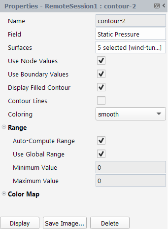
Specify all of the required fields in the Properties - RemoteSessionX: <graphics object name>.
Click Display at the bottom of the properties panel
Note: You can remove a graphics object from the remote client session by right-clicking it in the Outline View tree and selecting Remove.
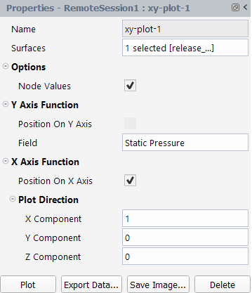
Click Actions ribbon tab (Plots group box).
Actions → Plots
→ New XYPlot...You can also create new plots objects by right-clicking XY Plots, in the Outline View tree and selecting New....
Specify all of the required fields in the Properties of RemoteSession-X: <plot object name>.
Click at the bottom of the properties panel.
(Optional) Click to open the Select File dialog and specify a location to save the plot data.
(Optional) Click to open the Save Picture Dialog Box in the Fluent User's Guide.
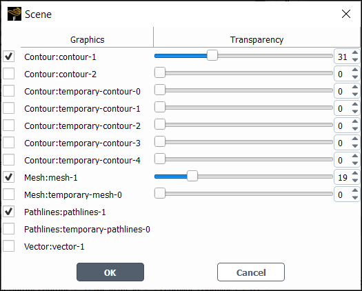
Scenes allow you to display multiple graphics objects within a single window. For example, you could overlay contours of pressure across a valve with velocity vectors and the mesh at the same location. Scenes allow you to modify the transparency of each plot so that you can emphasize a particular plot or view.
To define a scene:
Create graphics objects to include in the scene, as described in Creating and Displaying Graphics objects.
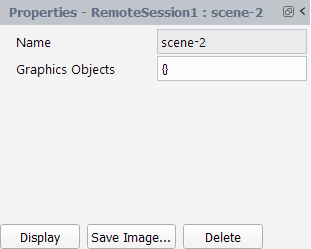
Right-click Scene in the Outline View tree and click New....
 Results → Scene
 New...
Click in the Graphics Objects field to open the Scene dialog box.
Enable the check boxes (on the left) for each of the graphics objects you want included in the scene.
(Optional) Adjust the transparency of contour and mesh plots using the Transparency slider.
Click to confirm the selections and close the dialog box.
Click at the bottom of the properties panel to display your scene in the graphics window.
Once you display a postprocessing object such as a contour, XY Plot, or Scene, you may want to save the image to a file.
To save an image to a file:
Open the properties panel for a postprocessing object.
Results → Graphics |
Plots → <graphics type>
→ <graphics object name>Click at the bottom of the properties panel to open the Save Picture Dialog Box in the Fluent User's Guide.
Specify your desired settings for saving the image and click to open the Select File dialog box.
Provide the location where you want the image saved and click .
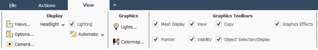
You can change how graphics objects are displayed in the graphics window of the Remote Visualization Client directly in the graphics window and via the Viewing ribbon tab.
When changes are made to graphics objects on the server or the client, there are options (available on a right-click of the object in the tree) to:
Send to server
sends changes made to the selected graphics object in the client to the server.
Retrieve from server
updates the graphics object in the client to match the state of the same object on the server.
View differences
prints the differences between the server and client versions of the graphics object to the console.
Arrows next to the graphics object indicate the state of the object. A single
upward-pointing arrow (![]() ) indicates that this graphics object is unique to the client. A
downward-pointing arrow paired with an upward pointing arrow (
) indicates that this graphics object is unique to the client. A
downward-pointing arrow paired with an upward pointing arrow (![]() ) indicates that the same object has different properties between the
server and the client.
) indicates that the same object has different properties between the
server and the client.
Note: Changes (new graphics objects and modified object settings) sent from the client to the server while the server is solving may not appear in the server until after the solving completes.
Fluent communicates with you when you are in the Remote Visualization Client through messages printed in the Console and the RemoteSession-X tabs. Generally, contents printed in the Console tab are related to the remote client session, but not necessarily to a specific remote server connection, whereas the RemoteSession-X tab(s) only apply to the server session that they are connected to. It is important to check both messaging tabs to ensure that you are getting all the information Fluent is sharing with you. The Console is also a Python 2.7 interpreter—refer to Python, Scripting and Transcripts in the Remote Client for additional information.
There are two ways that you can enter text commands from the Fluent Remote Visualization Client.
Through the console—only controls the client session (no effect on the server) and provides options to exit the session and modify the views.
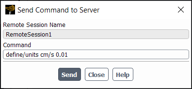
Through the Send Command to Server dialog box—sends commands to the server. This option offers all of the commands listed in the Fluent Text Command List.
Important: Do not start calculations from the Send Command to Server dialog box—they must be started using the GUI on the client.
Note: If the server is running with the active GUI present, some commands, such as changing the discretization scheme, may require a refresh of the task page displaying the effected field on the server (Solution Methods in the example of a modified discretization scheme) before the change appears in the GUI—the changed field is still applied even if you do not update the GUI display.
To send text commands to the server:
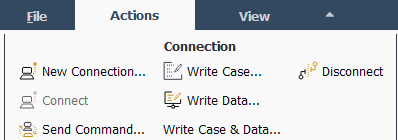
Open the Send Command to Server dialog box by clicking in the Actions ribbon tab (Connection group box).
Actions → Connection
→ Send Command...Enter the text command into the Command text entry box.
Note: If you want the text command to be run in the background without the client waiting for it to complete, then you can add an
&to the end of the command. For example,define/units velocity cm/s 0.01&.Click .
Important:
While Fluent is solving, do not enter any commands that modify Fluent, such as changing equations, plots, models, and so on, as this could cause errors.
Ensure that you only enter complete TUI commands in the Send Command to Server dialog box.
Confirm that you are sending the command to the intended server if you are connected to multiple servers. The remote session that is sending the command is listed under Remote Session Name. Select a remote session in the tree to review its properties, which includes the name of the host machine (server).
As noted in the Warning dialog box that appears, commands are executed immediately in the solver session without confirmation. This could cause a loss of work, if other users are connected to and modifying the same session as you.
For any actions sent from the Remote Visualization Client to the server (initialization, starting calculation, text commands using Send Command to Server), text prompts are automatically answered. For example, if the question is The current data has not been saved. OK to discard? Ansys Fluent automatically answers OK to this question and begins calculating.
You can write case and data files from the client.
![]() Actions → Connection
→ Write Case... | Write Data... | Write Case &
Data...
Actions → Connection
→ Write Case... | Write Data... | Write Case &
Data...
Writing a case and/or data file:
Click Write Case..., Write Data..., or Write Case and Data....
Enter the name and location where the file(s) will be saved in the File name field.
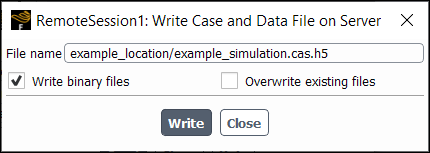
(Optional) Enable Write binary files to write binary files instead of text files. Binary files take up less space and Fluent can read them and write them faster than text files.
(Optional) Enable Overwrite file if exist if you want Fluent to write the new case and/or data files, even if this means overwriting existing files with the same name in the location that you specified.
Click to save the file(s).
If you want to break a server-client connection you can accomplish this in two ways: from within the client and from within the server.
Note: If the server is closed unexpectedly, for example, the process is ended from the Windows Task Manager, the remote visualization client may appear to hang, however after a time out the client will become responsive again.
To disconnect from within the client:
Select the RemoteSession-X connection that you want to break in the tree.
Click Disconnect in the Actions ribbon tab (Connection group box).
Actions → Connection
→ DisconnectYou can also disconnect the session by right-clicking the RemoteSession-X branch in the tree and selecting Disconnect.
Important: Do not try to close the server via the exit command in the
Send Command to Server dialog box, the correct command is
(exit-server).
To disconnect a client from within the server you must shutdown the server.
Shut down the server by selecting Shutdown Server in the File ribbon tab.
![]() File → Applications
→ Server → Shutdown
File → Applications
→ Server → Shutdown
You can also shutdown the server by entering the
server/shutdown-server
text command in the console.
You can control system preferences from the Remote Visualization Client in the same manor as described in Setting User Preferences/Options in the Fluent User's Guide.
![]() File → Preferences...
File → Preferences...
In addition to editing preferences through the GUI, you can also modify them through the
Python console. For example, you can set the graphics color theme to Gray
Gradient by entering
Preferences.Appearance.GraphicsColorTheme="Gray Gradient" and you
can enable Boundary Markers by entering
Preferences.Graphics.BoundaryMarkersEnabled="True". Refer to
Python, Scripting and Transcripts in the Remote Client for additional information on the Python console.
Note: If you want to know the valid inputs for a certain field, enter
Preferences.<BranchName>.<settingName>.getAttribValue('allowedValues').
For example,
Preferences.Appearance.GraphicsColorTheme.getAttribValue('allowedValues')
returns ['Workbench', 'Gray Gradient', 'White',
'Black'].