The following section describes the possible ways to interact with and post process the results of a Fluent Aero simulation.
During and after the Fluent Aero simulation, the Convergence window can be used to display the convergence plots of as well as any monitors such as , and . The Convergence window is shown by default when you begin a calculation. It is located in the same location as the Graphics window, and can be accessed at any time by selecting the Convergence tab.
The image below shows a Convergence window showing the of .
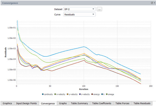
There are two items that can be used to control the content displayed in the Convergence plot window:
Dataset
Select the that you would like to see the or Monitors. Any that has been simulated will appear in the list of selectable .
Curve
Select the or Monitors of the selected. , , and pitch-, yaw- and roll-moment-coefficient are always available as selections in this menu when using Fluent Aero. Individual solver residuals and other solution monitors may also be available depending on your settings. For example, if a mixture has been selected for Air Properties, the residuals of each species will be available.
The convergence plots can be interacted with in the following ways:
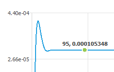
Display the value of a point on the curve
The value of a point on a curve can be displayed by clicking a curve near the point of interest.
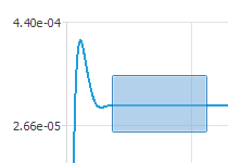
Zoom into a part of the curve
A section of the curve can be investigated further by zooming onto it using a Shift++.
Once a Fluent Aero simulation begins to calculate, a Results component menu will appear at the end of the Outline View tree. The Results component menu contains a Simulation and a Design Point sub-components that can be used to post process the results.
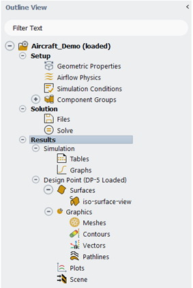
The Simulation component provides a comprehensive view of aerodynamic coefficients across all design points, which can be visualized using tables or graphs.
The Tables component contains commands to display tabulated results of a simulation. These commands are accessible by right-clicking Tables in the Outline View window, or by using a selectable dropdown list or buttons in the Properties - Tables window.
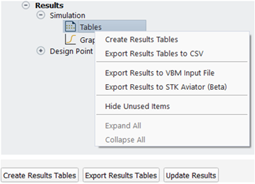
This function will create a set of results tables called Table:Summary, Table:Coefficients, Table:Forces, Table:Residuals, and if required, Table:Custom Output and Table:Component Output in the same area as the Graphics window. This table presents selected input and output values associated with each design point that was calculated in the simulation.
/
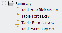
This function will export the results tables using comma separated values files Table-Coefficients.csv, Table-Forces.csv, Table-Residuals.csv and Table-Summary.csv located in a Summary folder inside Results.
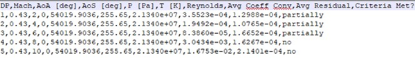
The following figure shows an example of Table-Summary.csv file to illustrate the file format used.
This function will export the results of aerodynamic coefficients to a .dat file which can be used as an input to describe the aerodynamic performance of an airfoil section of Fluent’s Virtual Blade Model (VBM).
After exporting this file, the file will be displayed in the Simulation → Results → Summary folder in the Project View, and stored in the Simulation → Results folder on disk.
File Format
The following image shows an example of the VBM input file created by Fluent Aero and annotated for clarity.
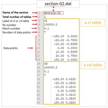
Header
At the top of the file, there is a short header, which contains:
The section name.
The number of tables inside the file.
Tables
Below the header is a cl and cd table for each combination of Mach and Reynolds number representing a group of design point results used in the simulation. Each table consists of the following:
cl or cd to specify which output values are contained in the subsequent table, representing a group of design point results.
The Reynolds number associated with the group of design point results.
The Mach number associated with the group of design point results.
The number of design points in the group of design point results.
Multiple lines containing the input angle of attack in degrees and output aerodynamic coefficient (cl or cd) for each design point in the group of design point results
File Requirements and Recommendations:
Fluent Aero will export results of a simulation using only the design points that are available in the simulation. However, care should be taken to ensure the simulation contains sufficient results to produce a viable VBM input file.
The data file must contain results for the full sweep of angles of attack, from -180 to 180 degrees for each group of design point results.
Note: Since an angle of attack of -180 degrees is equivalent to +180 degrees, only one of these should be calculated for each group of design points. The results will automatically fill both positions in the design point table.
A higher concentration of design points is recommended for angles of attack that could more commonly be used in VBM simulations or feature more significant changes in results with small increments in angle of attack.
This function will export the results of aerodynamic coefficients to a simple format .aero file supported by STK Aviator. This file can be used to define the aerodynamic performance of an aircraft during an AGI STK Aviator simulation.
This is currently a Beta feature, and it’s documentation can be found here Fluent Aero – Export Results to STK Aviator.
Refer to the STK Help at https://help.agi.com/stk/ for more information on how a .aero file can be used in STK Aviator.
This function will display the Table:Forces and Table:Coefficients tables based on the coordinate system selected by the user. Currently, the body-fixed and wind-fixed coordinate systems are supported for displaying aero forces and moments, along with their coefficients. The body-fixed axes are attached to the object and move with it; however, the wind-fixed axes are fixed with respect to the surrounding air. In both body-fixed and wind-fixed coordinate systems, the origin is the same; however, their orientations differ from each other due to the angle of attack and sideslip.
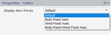
This option displays the lift and drag forces and coefficients in the wind-fixed coordinate system, and moment forces and coefficients in the body-fixed coordinate system. Typically, moments are calculated in the body-fixed axes. Therefore, body-fixed axes moments have been added to the default table in addition to the lift and drag. Gray color is used to differentiate the body-fixed axes coefficients from the wind-fixed axes coefficients.
Note: The lift and drag forces, along with the rolling, pitching, and yawing moments, have been computed within the Fluent Solution workspace during the simulation because these parameters are used to monitor the convergence.
This option displays all forces and moments, along with their coefficients, in the body-fixed coordinate system.
To obtain the body-fixed axial, side, and normal forces, the global x-, y-, and z-force components will be projected onto the axial, side, and normal force directions. Specifically, the axial direction will be derived from the user’s input of the drag direction at an AoA of 0 degrees. The normal direction will be determined by the user’s input of the lift direction at an AoA of 0 degrees. These directions are defined under Geometric Properties panel based on the orientation of the geometry. Additionally, the side force direction will be obtained by applying the right-hand rule to the cross-product of the normal and axial directions.
This option displays forces and moments, along with their coefficients, in the wind-fixed coordinate system.
In addition to the lift and drag forces, the crosswind force will be determined by projecting the global x-, y-, and z-force components onto the crosswind direction. To obtain the wind-fixed rolling, pitching, and yawing moments, the global x-, y-, and z-moment components will be projected onto the drag, crosswind, and lift force directions. The drag, crosswind, and lift directional vectors will be obtained from the global-to-body-fixed axes transformation matrix and then from the body-fixed-to-wind-fixed axes transformation matrix, which is called the directional cosine matrix (DCM) and is given by the following expression:
In the transformation matrix T, α is angle of attack and β is sideslip angle.
Body-Fixed+Wind-Fixed Axes
This option displays forces and moments, along with their coefficients, in both the body-fixed and wind-fixed coordinate systems simultaneously.
Note: The displayed tables of forces and moments on the screen, along with their coefficients, will be written to the files Table-Coefficients.csv and Table-Forces.csv when right-clicking on Tables in the Outline View window and selecting the option.
If you have changed a workflow setting that effects some of the tabulated results or has added a new custom output parameter, can be used to update all the results inside these tables without re-calculating each design point. For example, if you would like to change the Reference length of a group of design point solutions that have already been obtained in order to update the aerodynamic coefficients, you can simply change the Reference Length inside Geometric Properties and use to update these coefficients such that they are computed with the new value of Reference Length.
Note: Clicking after adding a new custom output parameter will cycle through each design point and load each solution file, so this process could take some time to complete, especially for larger cases.
There are four tables produced by Fluent Aero to help post-process the results: Table:Summary, Table:Coefficients, Table:Forces, Table:Residuals, and if required, Table:Custom Outputs and Table:Component Outputs.
Table:Summary
An example of Table:Summary is provided below along with a description of each item in the table.
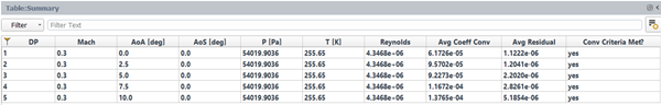
DP
The design point number associated with the row in the table.
Mach
The Mach number used to calculate the design point.
AOA [deg.]
The angle of attack used to calculate the design point.
P [Pa]
The static pressure used to calculate the design point.
T [K]
The static temperature used to calculate the design point.
Reynolds
The Reynolds number associated with design point flight conditions.
Avg. Coeff. Conv.
This value is the average of the convergence of the lift coefficient, drag coefficient and moment coefficient at the final iteration computed for the design point.
Avg. Residual
This value is the average of all residuals (from Table:Residuals) at the final iteration computed for the design point.
Criteria Met?
This value will list yes if the Cl and Cd Coefficients Convergence (Cl. Conv. and Cd. Conv.) (from Table:Coefficients) and all Residuals (from Table:Residuals) meet their respective convergence conditions specified in Solve → → Aero Convergence Cutoff (default 1e-5) and Aero Coeff. Convergence Cutoff (default 2e-5). It will list no if these conditions have not been met, partially if some of the conditions have been met, and diverged if the design point calculation stopped early due to divergence of a calculation.
Note: The convergence of the Cm-y, Cm-p, and Cm-r values (partially reported in the Max. Cm Conv. column) are not used to determine if the convergence criteria is met. If interested, you should investigate these values manually with the Max. Cm Conv. value in the table or using the Convergence graphs.


Table:Coefficients
An example of Table:Coefficients is provided below along with a description of each item in the table when the option has been selected under Display Aero Forces. Gray color is used to differentiate the body-fixed axes coefficients from the wind-fixed axes coefficients.
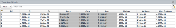
DP
The design point number associated with the row in the table.
Cl
The Lift Coefficient computed for the design point. This coefficient considers the pressure and shear forces on all walls in the geometry.
Cd
The Drag Coefficient computed for the design point. This coefficient takes into account the pressure and shear forces on all walls in the geometry.
Cm-y
The body-fixed Yaw Moment Coefficient computed for the design point. This coefficient considers the pressure and shear forces on all walls in the geometry.
Cm-p
The body-fixed Pitch Moment Coefficient computed for the design point. This coefficient takes into account the pressure and shear forces on all walls in the geometry.
Cm-r
The body-fixed Roll Moment Coefficient computed for the design point. This coefficient considers the pressure and shear forces on all walls in the geometry.
Cl Conv.
A value measuring the convergence of the lift coefficient at the final iteration computed in the simulation of the design point. This value is computed using the following equation,
where
is the lift coefficient at the final iteration, and
is the lift coefficient that produces the maximum difference when compared to
from among the most recent previous iterations. By default, the 10 most recent iterations are used. To specify a different value, go toSolve and set Convergence Criteria to Custom. Then you can modify the value under Solve→ Convergence Criteria → Aero Conv. Coeff Previous Values
Note: In some situations, when the absolute value of
 is very low (for example, when
simulating a symmetrical airfoil at an angle of attack
of 0 degrees), the value of Cl
Conv. as computed in the above equation
would be high, even when the solution is well converged.
To give a more meaningful value of Cl
Conv. for these situations, if the value
of
is very low (for example, when
simulating a symmetrical airfoil at an angle of attack
of 0 degrees), the value of Cl
Conv. as computed in the above equation
would be high, even when the solution is well converged.
To give a more meaningful value of Cl
Conv. for these situations, if the value
of  is less than
Solve →
Convergence Criteria(set as
Custom) → Aero
Coeff Conv. Cutoff, the following
equation is used instead:
is less than
Solve →
Convergence Criteria(set as
Custom) → Aero
Coeff Conv. Cutoff, the following
equation is used instead: Cd Conv.
A value measuring the convergence of the drag coefficient at the final iteration computed in the simulation of the design point. This value is computed using the following equation,
where
is the drag coefficient at the final iteration, and
is the drag coefficient that produces the maximum difference when compared to
from among the most recent previous iterations. By default, the 10 most recent iterations are used, and this can be specified in Solve → → Aero Conv. Coeff Previous Values.
Max Cm Conv.
A value measuring the convergence of the moment coefficients at the final iteration in the simulation of the design point. This value is computed using the following equation,
(Cmy, Cmp, Cmr) is each moment coefficient at the final iteration, and each
is the moment coefficient that produces the maximum difference when compared to each
from among the most recent previous iterations. Therefore, the Max Cm Conv. value in the table will show the moment coefficient with the highest value. By default, the 10 most recent iterations are used, and this can be specified in Solve → → Aero Conv. Coeff Previous Values.
An example of Table:Coefficients is provided below along with a description of each item in the table when the option has been selected under Display Aero Forces.
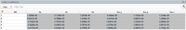
DP
The design point number associated with the row in the table.
Ca
The Axial Force Coefficient computed for the design point. This coefficient considers the pressure and shear forces on all walls in the geometry.
Cs
The Side Force Coefficient computed for the design point. This coefficient takes into account the pressure and shear forces on all walls in the geometry.
Cn
The Normal Force Coefficient computed for the design point. This coefficient takes into account the pressure and shear forces on all walls in the geometry.
Cm-y
The body-fixed Yaw Moment Coefficient computed for the design point. This coefficient considers the pressure and shear forces on all walls in the geometry.
Cm-p
The body-fixed Pitch Moment Coefficient computed for the design point. This coefficient takes into account the pressure and shear forces on all walls in the geometry.
Cm-r
The body-fixed Roll Moment Coefficient computed for the design point. This coefficient considers the pressure and shear forces on all walls in the geometry.
An example of Table:Coefficients is provided below along with a description of each item in the table when the option has been selected under Display Aero Forces.
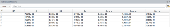
DP
The design point number associated with the row in the table.
Cl
The Lift Coefficient computed for the design point. This coefficient considers the pressure and shear forces on all walls in the geometry.
Cd
The Drag Coefficient computed for the design point. This coefficient takes into account the pressure and shear forces on all walls in the geometry.
Cc
The Crosswind Force Coefficient computed for the design point. This coefficient takes into account the pressure and shear forces on all walls in the geometry.
Cm-y
The wind-fixed Yaw Moment Coefficient computed for the design point. This coefficient considers the pressure and shear forces on all walls in the geometry.
Cm-p
The wind-fixed Pitch Moment Coefficient computed for the design point. This coefficient takes into account the pressure and shear forces on all walls in the geometry.
Cm-r
The wind-fixed Roll Moment Coefficient computed for the design point. This coefficient considers the pressure and shear forces on all walls in the geometry.
Table:Forces
An example of Table:Forces is provided below along with a description of each item in the table when the option has been selected in the dropdown list of Display Aero Forces. Gray color is used to differentiate the body-fixed axes data from the wind-fixed axes data.
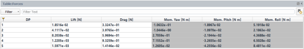
DP
The design point number associated with the row in the table.
Lift [N]
The total Lift force computed for the design point. This force takes into account the pressure and shear forces on all walls in the geometry.
Drag [N]
The total Drag force computed for the design point. This force takes into account the pressure and shear forces on all walls in the geometry.
Mom. Yaw [N.m]
The body-fixed total Yaw Moment force computed for the design point. This force takes into account the pressure and shear forces on all walls in the geometry.
Mom. Pitch [N.m]
The body-fixed total Pitch Moment force computed for the design point. This force takes into account the pressure and shear forces on all walls in the geometry.
Mom. Roll [N.m]
The body-fixed total Roll Moment force computed for the design point. This force takes into account the pressure and shear forces on all walls in the geometry.
An example of Table:Forces is provided below along with a description of each item in the table when the option has been selected under Display Aero Forces.
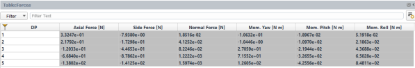
DP
The design point number associated with the row in the table.
Axial Force [N]
The total Axial Force computed for the design point. This force takes into account the pressure and shear forces on all walls in the geometry.
Side Force [N]
The total Side Force computed for the design point. This force takes into account the pressure and shear forces on all walls in the geometry.
Normal Force [N]
The total Normal Force computed for the design point. This force takes into account the pressure and shear forces on all walls in the geometry.
Mom. Yaw [N.m]
The body-fixed total Yaw Moment force computed for the design point. This force takes into account the pressure and shear forces on all walls in the geometry.
Mom. Pitch [N.m]
The body-fixed total Pitch Moment force computed for the design point. This force takes into account the pressure and shear forces on all walls in the geometry.
Mom. Roll [N.m]
The body-fixed total Roll Moment force computed for the design point. This force takes into account the pressure and shear forces on all walls in the geometry.
An example of Table:Forces is provided below along with a description of each item in the table when the option has been selected under Display Aero Forces.
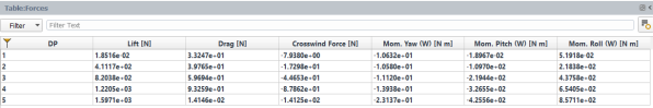
DP
The design point number associated with the row in the table.
Lift [N]
The total Lift force computed for the design point. This force takes into account the pressure and shear forces on all walls in the geometry.
Drag [N]
The total Drag force computed for the design point. This force takes into account the pressure and shear forces on all walls in the geometry.
Crosswind Force [N]
The total Crosswind Force computed for the design point. This force takes into account the pressure and shear forces on all walls in the geometry.
Mom. Yaw (W) [N.m]
The wind-fixed total Yaw Moment force computed for the design point. This force takes into account the pressure and shear forces on all walls in the geometry.
Mom. Pitch (W) [N.m]
The wind-fixed total Pitch Moment force computed for the design point. This force takes into account the pressure and shear forces on all walls in the geometry.
Mom. Roll (W) [N.m]
The wind-fixed total Roll Moment force computed for the design point. This force takes into account the pressure and shear forces on all walls in the geometry.
Table:Residuals
An example of Table:Residuals is shown below. The residual names listed may change depending on the models that are used in your simulation.
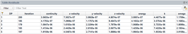
Table:Custom Outputs
An example of Table:Custom Outputs is shown below. The custom ouputs listed will change depending the custom outputs selected in the Simulation Conditions → panel.
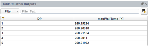
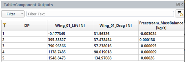
Table:Component Outputs
An example of Table:Component Outputs is shown below. The component ouputs listed will change depending the group types that are used in Component Groups and the outputs selected in the Manage Component Outputs panel. The names of the component outputs in the table header will contain both the group name and the variable name.


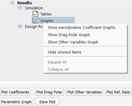
The Graphs component contains commands to display aerodynamic coefficient plots using the results of your simulations inside the Graphics window. These commands are accessible by right-clicking Graphs in the Outline View, or as buttons located at the bottom of the Graphs properties window.
/
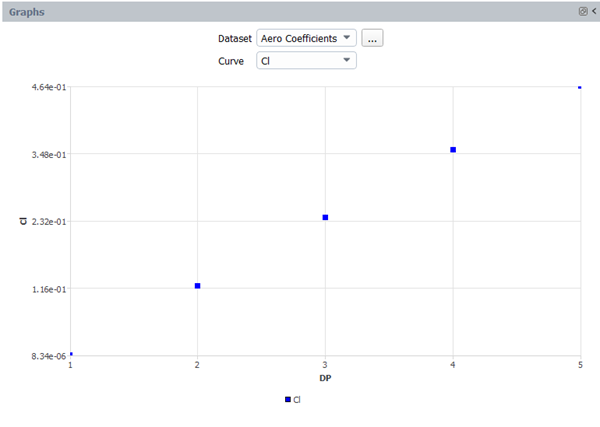
This function will cause the graphics window to present the Graphs window showing the aerodynamic coefficients with respect to the design point number for all design points that were calculated in the simulation. The Dataset will be set to , which uses data stored in the Tables-Coefficients.csv file in the simulation’s Results folder.
Below is an example of Graphs panel showing a Coefficient graph when the Default option is selected under Tables->Display Aero Forces. The y-axis definition can be modified by making a selection from the Curve selection box at the top of the graph. , , , and can be selected. If the Body-Fixed Axes or option is selected under Tables->, , and become available.
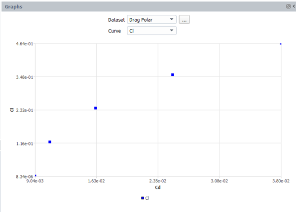
This function will cause the graphics window to present the lift coefficient with respect to the drag coefficient for all design points that were calculated in the simulation. The Dataset will be set to , which uses the Table-ClCd.csv file in the simulation’s Results folder. An example of Graphs panel showing a Drag Polar, Cl vs. Cd graph is shown below.
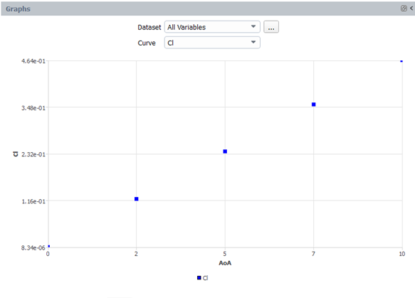
Plot Other Variables / Show Other Variables Graphs
This function will cause the graphics window to present the Graphs window where you create a graph of any input or output parameters (including custom inputs and outputs) that were used in the simulation. The Dataset will be set to the Table-All.csv file in the simulation’s Results folder. In this mode, it is useful to use the […] options selection panel to have additional control over the x-axis and y-axis variables for example, you could plot the Cl vs. Angle of Attack using this plot set.
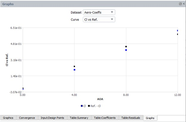
This function will open a file navigation window where a comma separated value (.csv) file containing reference data can be selected. This file will be then read and its content added to the active graph panel.
The .csv file must be formatted such that the first line contains the x-axis value (either AOA, Mach or DP) and the y-axis value (either Cl, Cd, Cm or Cl/Cd) separated by a comma. The remaining lines of the file can contain the reference data points. An example .csv reference data file and associated Graphs panel is shown below.
Note: The file should be formatted such that there are no spaces between each header variable or data value.

This function will save the content of the Graphs panel to a .png image file on the disk.
Parametric Graph
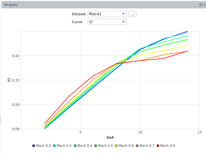
This function will open a Parametric Graph panel, where you can setup and plot a parametric plot using the outputs for each design point. The Parametric Graph panel contains additional controls that are useful for creating graphs to compare more complex datasets with larger numbers of design points.

Once you select the Parametric Graph settings, and click , a new plot will appear in the Graphs panel. The settings in the above image could result in a plot similar to the below:
The following options can be used to construct a Parametric Graph:
Plot Name
Name
Set the name of the parametric graph.
Plot Variables
Group by
Select the variable to use to group the outputs parameters into groups of curves. For each different value of the Group, a curve group will be created in the parametric plot. For example, if Group by is set to , and 3 different Mach numbers were used in the input design points, there will be 3 groups of curves shown in the parametric plot, each labeled by their respective Mach number.
x-variable
Select the variable to plot on the x-axis of the parametric graph.
y-variable
Select the variable to plot on the y-axis of the parametric graph.
Options
Exclude DPs
Select certain design points to exclude from the plot. Design points can be excluded by the convergence status (, ), as shown in the Criteria Met? column of the input table. Alternatively, a Custom set of design points can be excluded.
List of DPs
Select a range of custom design points to be excluded. Commas (,) and hyphens (-) can be used to control the range of design points to be excluded. For example, entering 1,3-5,10 will exclude design points 1, 3, 4, 5 and 10.
Number of Filters
Set a number of filters to use to filter in and out design points with certain parameter values from the Parametric Graph.
Each filter can be controlled using the Active, Variable, Minimum Value and Maximum Value settings. Set a filter to Active to enable that specific filter. Set the Variable to the parameter for which you would like to filter the results. Set the Minimum Value and Maximum Value to control the range of values for that parameter that you would like to include in the plot.
For example, if you enter an Active filter using the Variable set to , the Minimum Value set to 0.9 and the Maximum Value set to 1.0, only design points with an input Mach number between 0.9 and 1.1 will be included in the Parametric Graph.
Curve Settings
Line/Scatter Style: Set a line or scatter plot style to use in the Parametric Graph.
Color: Set the color pallet to use in the Parametric Graph.
: Select this to plot the requested Parametric Graph in the Graphs window.
: This function will open a file navigation window where a comma separated value (.csv) file containing reference data can be selected. This file will be then read, and its content added to the active graph panel.
The .csv file should be formatted such that at least all variables selected for the Group by x-variable and y-variable are included in the file. The first line header should contain the variable names, separated by commas. The remaining lines of the file can contain the reference data points. Only the variables with a first line header name that is the same as any referenced in the Parametric Graph control panel will be used. However, the file can contain additional variables, but they will not be used in the plot.
Note: The file should be formatted such that there are no spaces between each header variable or data value.
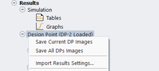
The Design Point component allows you to review the results specific to an individual design point in the graphics window. You can visualize objects such as meshes, contours, vectors, pathlines, XY plots and scenes. You can also create surfaces for further exploration. The component also includes commands to load results for a design point and save graphic images for the current or all updated design points.
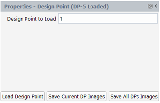
Load Design Point
This function allows you to load the solution of the design point specified under Design Point to Load.
Save Current DP Images
This function allows you to save all graphic images for the current design point. Any graphic results with the Save Image option enabled will be saved as an image. Settings from the properties panel, including the specified view and save image options will be respected. The progress of saving images will be displayed both on the progress bar and within the console.
Save All DPs Images
This function can be used to save images for all updated design points. Similar to the above function, it saves graphics results with the Save Image option enabled and respects settings from the properties panel. The progress of saving images will be displayed both on the progress bar and in the console.
When you execute the Save Current DP Imagesor Save All DPs Images command, the images are registered inside the ProjectView -> Results -> DP-# -> Data folder. However, these images are hidden by default and can be shown by clicking on Project -> ViewOptions -> ShowHiddenItems from the Fluent Aero ribbon.
The properties panel or right-click menu of a graphics object under Design Point in the outline view tree provides the following commands for efficient management of graphics objects:
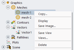
Copy...
This command creates a duplicate of an existing graphics object, eliminating the need to reapply all settings.
Display
This command allows you to display the selected graphics object in the Graphics window.
Save Image...
This command opens the Save Picture dialog box where you can save an image file of the object with the specified options. For more details, please refer to Save Picture Dialog Box. The Apply button saves the specified options, which will be automatically applied when you save images using the Save Current DP Images or Save All DPs Images command.

Save View
After displaying the graphic object in the Graphics window and adjusting the view, this command allows you to save it. The view is stored under View inside the properties panel, with the view name formatted as aero-view-<graphic-object-name>. The saved view is automatically applied when you click Display or use the Save Current DP Images and Save All DPs Images commands with the Save Image option enabled.
Views...
This command opens the Views dialog box, where you can manage the views for your graphics results. For more details, please refer to Views Dialog Box.
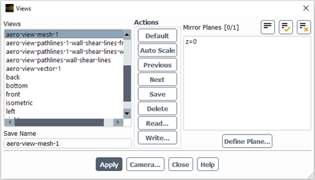
Note: When using Save Current DP Images or Save All DPs Images commands, please note that the part of image that is created from applying a mirror plane will not be saved.
Delete
This command deletes the selected graphics object.
You can create different types of surfaces to visualize your results, including points, lines, rakes, planes, and iso-surfaces. To create and visualize a graphic object, follow these steps:
Click New then select Point..., Line..., Rake..., Plane... or Iso-Surface... to create a new point, line, rake, plane or iso-surface.
 Results→Design Point
→Surfaces→ New
→ Point...
or Line... or
Rake... or Plane... or
Iso-Surface
Results→Design Point
→Surfaces→ New
→ Point...
or Line... or
Rake... or Plane... or
Iso-SurfaceSpecify all the required fields in the properties panel of the new surface object that appears. For details on each setting, refer to Surfaces.
Click Display to visualize the surface object in the Graphics window. Commands such as Save Image… and Delete allow you to either save the plot or delete a surface. For more details on each command, refer to the beginning of Design Point
Note:
To ensure updated surface definitions (for example, if you change the location of a line) are properly shown when included in a scene or other graphics object, display the surface before re-displaying the containing object.
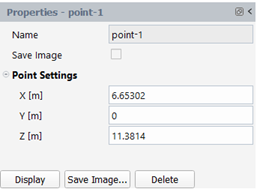
Point
This allows you to display results at a single point in the domain. For instance, you can monitor the value of a specific variable at a particular location. When you display node-value data on a point, the value displayed is a linear average of the neighboring node values. If you display cell-value data, the value at the cell in which the point lies is displayed.
The figure below shows the Properties panel of a point object. For details on each setting, refer to Point Properties
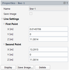
Line
A line is a straight segment that extends up to and includes the specified endpoints; data points will be located where the line intersects the faces of the cell, and consequently may not be equally spaced.
The figure below shows the Properties panel of a line object. For details on each setting, refer to Line Properties
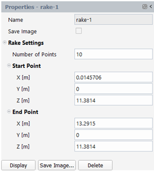
Rake
A rake consists of a specified number of points equally spaced between two specified endpoints.
The figure below shows the Properties panel of a rake object. For details on each setting, refer to Rake Properties
Plane
A plane surface allows you to visualize flow-field data on a specific plane within the domain. You can create surfaces that cut through the solution domain along arbitrary planes.
The figure below shows the Properties panel of a plane surface. For details on each setting, refer to Plane Properties
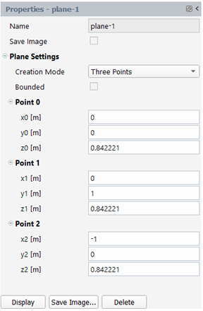
There are three types of plane surfaces that you can create (via the Creation Mode):
Coordinate system-based: The plane is created in the YX, ZX, or XY directions, bounded by the domain’s extents. You can move the plane to the desired location in the domain using the plane tool. For example, if you are using the YZ Plane method, you can drag the plane in the (+) or (-) X direction.
Point and normal: The plane orientation is determined by selecting a point and specifying a direction normal to that point. The plane’s edges correspond to the domain’s boundaries. You can control the orientation using the plane tool or compute the normal from a surface.
Three points—the orientation and extends of the plane are determined by three selected points and domain boundaries. You can directly manipulate the points and orientation of the plane in the graphics window using the plane tool.
Creating Multiple Planes
Instead of creating plane surfaces one at a time as described above, you have the option to create multiple plane surfaces at once using the Create Multiple Planes Dialog Box:
![]() Results→Design Point →Surfaces→ Create Multiple
Planes...
Results→Design Point →Surfaces→ Create Multiple
Planes...
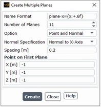
To use the Create Multiple Planes dialog box:
(Optional) Provide a format for naming the plane surfaces in the Name Format field.
Specify how many planes will be created in the Number of Planes field.
Select the method for how you want to create the planes in the Option drop-down list.
Point and Normal—similarly to the process described earlier in this section, you must provide a point and the direction normal to that point to define the first plane.
First and Last Point—you define the coordinates for the first and last point, which determines the orientation of the planes. The spacing is determined by how many planes you specify in the Number of Planes field.
(Point and Normal only) Specify the direction normal (perpendicular) to the plane in the Normal Specification drop-down list.
(Point and Normal only) Specify how far apart the planes are from each other in the Spacing field.
Provide the coordinate for the location of the first plane in the Point on First Plane group box.
(First and Last Point only) Provide the coordinates for the location of the last plane in the Point on Last Plane group box.
Click Create to create the new plane surfaces.
The new plane surfaces created using the Create Multiple Planes dialog box are added to the OutlineView tree under the Surfaces and are now eligible for editing individually.
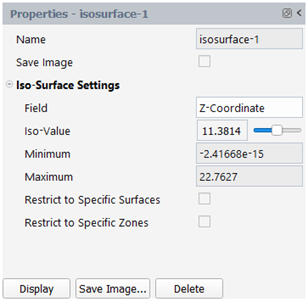
Iso-Surfaces
Iso-Surfaces can be used to display results on cells that have a constant value for a specified variable. For example, generating an iso-surface based on x, y-, or z- coordinate will give you an x, y, or z cross-section of your domain; generating an iso-surface based on pressure will enable you to display data for another variable on a surface of constant pressure. You can create an iso-surface from an existing surface or from the entire domain. Furthermore, you can restrict any iso-surface to a specified cell zone.
The figure below shows the Properties panel of an iso-surface. For details on each setting, refer to Iso-Surface Properties
This section describes the various graphic objects available in Fluent Aero, including meshes, contours, vectors and pathlines. To create and visualize a graphic object, follow these steps:
Click the New… command, either on the properties panel or in the right-click menu of a graphic object node (Meshes, Contours, Vectors, Pathlines) under Results -> Design Point -> Graphics
Results→Design Point →Graphics→Meshes
or Contours or Vectors or Pathlines  New....
Specify all the required fields in the properties panel of the new graphic object that appears. For details on each setting, refer to Graphics.
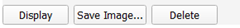
Click Display to visualize the graphic object in the Graphics window. Additionally, commands such as Save Image…,Delete, Copy…, Save View and Views… are available for managing and saving graphics objects. These commands can be found either at the bottom of the properties panel or in the right-click menu. For more information on each command, refer to the beginning of section Design Point.
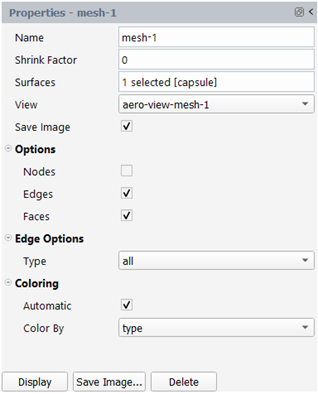
Meshes
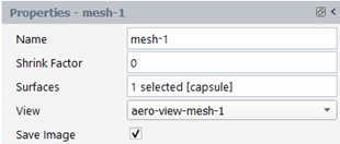
Mesh objects can be generated to display all or part of the mesh, or to create other graphic objects such as contours or scenes.
The figure below shows the Properties panel of a mesh object. For details on each setting, refer to Mesh Properties.
Contours
The Contours component contains commands to display 3D contour plots of results of a simulation in the Graphics window.
The figure below shows the Properties panel of a contour object. For details on each setting, refer to Contour Properties
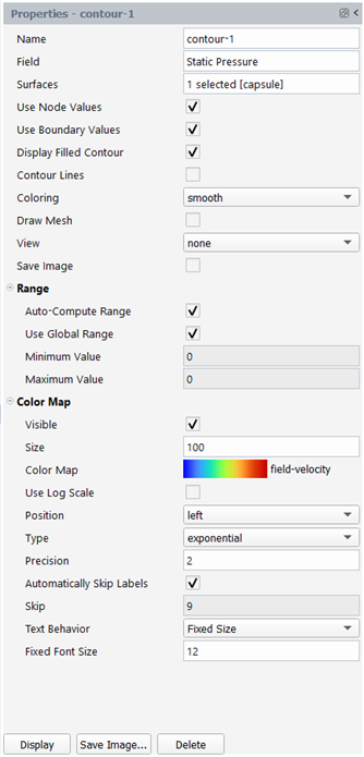
Alternatively, you can create a contour directly from the properties panel of Contours. When you click on the Contours item, the Properties – Contours panel will appear. The first setting in this panel is Surfaces, which has four options: Walls, Component Groups, Selected Surfaces, and Cutting Plane. The settings available on the properties panel will change based on the option you select. Settings such as Field, Auto-Compute Range, Draw Mesh and Color Map are the same as for contour objects. For more details on these settings, please refer to Contour Properties
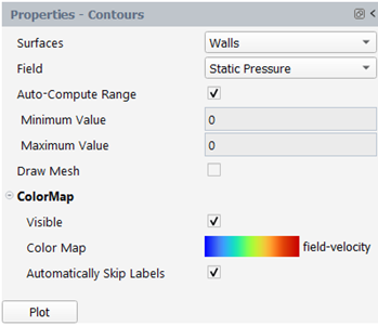
Surfaces – Walls
When Surfaces is set to Walls in Properties – Contours, a contour will be plotted on all wall boundaries in the domain and the following options are available:
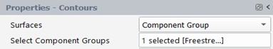
Surfaces – Component Group
When Surfaces is set to Component Group in Properties- Contours, one extra option is available where you can Select Component Groups to be displayed:
Surfaces – Cutting Plane
When Surfaces is set to Cutting Plane in Properties – Contours, three additional options become available to plot a contour on a cutting plane in the Graphics window. This cutting plane will be coplanar to the lift and drag direction vectors setup in Geometric Properties.
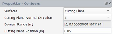
Cutting Plane Normal Direction
This represents the normal direction of your cutting plane, which is restricted to Cartesian axis directions.
Domain Range [m]
This value shows you the minimum and maximum grid positions the cutting plane can be set to.
Cutting Plane Position [m]
This specifies the grid position of the cutting plane that will be used for contour plotting.
Once you have set all the settings, you can create the contour by clicking on the Plot button. A contour object will be created under Contours and displayed in the Graphic window.
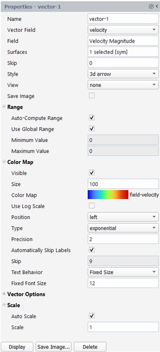
Vectors
You can draw vectors in the entire domain, or on selected surfaces. By default, one vector is drawn at the center of each cell (or at the center of each facet of a data surface), with the length of the arrows represented by the selected vector field and the color of the arrows represented by the selected scalar field. The spacing, size, and coloring of the arrows can be modified, along with several other vector plot settings. Note that cell-center values are always used for vector plots; you cannot plot node-averaged values.
The figure below shows the Properties panel of a vector object. For details on each setting, refer to Vector Properties
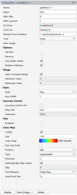
Pathlines
Pathlines are used to visualize the flow of massless particles in the problem domain. The particles are released from one or more surfaces that you have created as described in Surfaces. A line or rake surface is most commonly used.
The figure below shows the Properties panel of a pathlines object. For details on each setting, refer to Pathlines Properties.
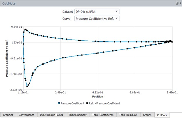
The Plots component contains commands to display 2D surface cut plots of results of a simulation in the Graphics window.
By default, the plane used to create the surface cut plots will be oriented coplanar with the Lift and Drag Direction Axis, as setup in the Grid Properties step.
Clicking the Plots item will cause the Plots properties window to appear.
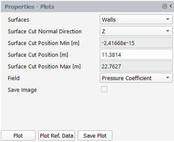
Surfaces
Defines the surface to use on which to display the surface cut 2D plot values. Choosing plots on all walls of the domain. Choosing will reveal another option where individual surfaces can be selected to use for the plot.
Surface Cut Normal Direction
Set the normal direction of the cut plane surface.
Surface Cut Position Min [m]
This value specifies the minimum global grid position, in meters, available in the direction normal to the plane that can be used to create the surface cut plot.
Surface Cut Position [m]
Specify the global grid position, in meters, where a surface cut plot will be plotted.
Surface Cut Position Max [m]
This value specifies the maximum global grid position, in meters, available in the direction normal to the plane that can be used to create the surface cut plot.
Field
Specify the field value to plot.
Note: When the two-temperature model is enabled or a mixture is selected for Air Properties, extra variables concerning the concentration of each species and the two-temperature model will become available.
Save Image
Enable to save the current plot when executing the Save Current DP Images or Save All DPs Images command.
This command will create the 2D surface cut plot in the Graphics window. If the design point number listed in the selection box is different than the solution that is currently loaded, the appropriate solution will be loaded before the plot is created.
An example Plot is shown below.
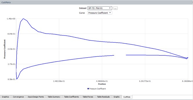
When is used, a comma separated value file is also created with the x-y data used to generate the plot. This file will be saved to a Data folder inside the design point folder associated with the solution used to generate the plot.
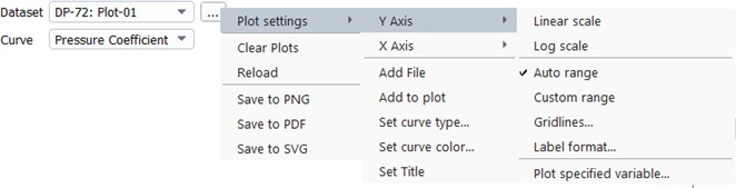
The graphics window will switch to the Plots tab, and the requested plot will be shown. At the top, the Dataset selection will show the name of the plot just generated (example: DP-72: Plot-01), starting with the design point number, and ending with the plot number. If multiple plots have been generated, one can click the drop-down list to select and display previously generated plots. The Curve selection will show the Y-axis variable that was used to generate the plot.
Additionally, a Plot Options window will appear which allows you to modify the line and the point plot display format to use for the plot. Modify any setting and click the button in the Plot Options window to update the plot format.
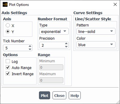
Additional controls of the Plot display can be performed using the […] options button located to the right of the dataset name. These controls can be used to save a picture of the plot to disk, change the X- and Y-Axis properties, add additional data to the plot, change the curve types, set plot titles, and more.
This function will open a file navigation window where a comma separated value (.csv) file containing reference data can be selected. The reference data will then be added to the active and representative graph panel.
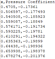
The .csv file must be formatted such that the first line header contains the cartesian axis used to plot the data – x, y, or z – followed by the y-axis variable (use the same name as it is listed in the y-axis of the plot) separated by a comma. The remaining lines of the file can contain the reference datapoints. An example of .csv reference data file and associated Graphs panel is shown below.
Note: The file should be formatted such that there are no spaces between each header variable or data value. When using Save Current DP Images or Save All DPs Images commands, please note that the reference data will not be included in the plot.
This function will save the content of the Graphs panel to a .png image file on the disk.
Note: The Plots component, detailed in this section, provides a streamlined approach for creating XY plots by combining the generation of 2D surface and XY plot into a single process. However, only one instance of XY Plot can be created. For situations that require the generation of multiple XY plots, consider activating and using the Fluent style Plots. For more details about how to activate and use the Fluent style Plots, please refer to Plots Properties.
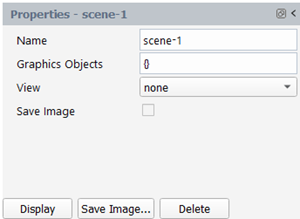
Scenes allow you to display multiple graphics plots within a single window. For example, you could overlay contours of pressure across a valve with velocity vectors and the mesh at the same location. Scenes allow you to modify the transparency of each plot so that you can emphasize a particular plot or view.
To create a scene, navigate to Results -> DesignPoint -> Scene and click New…. Go to the Properties panel of the scene object to specify the settings. For details on each setting, refer to Scene Properties
![]() Results→Design Point →Scene
Results→Design Point →Scene
![]() New...
New...
Once all the settings are defined, click Display to show the scene plot in the Graphics window. Additionally, commands such as Save Image…,Delete, Copy…, Save View and Views… are available for managing and saving a scene object. These commands can be found either at the bottom of the properties panel or on the right-click menu. For more information on each command, refer to the beginning of section Design Point.
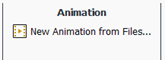
The Fluent Aero interface includes a tool allows you to create animations from image files. This tool can be accessed from the Results -> Animation section of the Fluent Aero ribbon.
To create a new animation from files, follow these steps:
Click on the New Animation from Files… button from the Results -> Animation ribbon section. This will open the Animation Options dialog box.
In the Animation Options dialog box, perform the following:
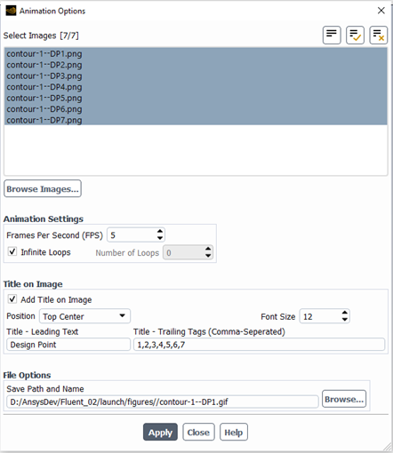
Select Images: Click Browse Images… to select the images for your animation. The order in which you select the images determines the order in which they appear in the animation.
Specify Animation Settings
Frames Per Second (FPS): Set the frames per second (FPS) for the animation.
Infinite Loops: Enable this option if you want the animation to play continuously.
Number of Loops: If the Infinite Loops option is disabled, specify the number of times the animation should loop.
Add Title on Image: Add a title to each image in the animation.
Add Title on Image: Check to add a title to each image.
Position: Choose where the title should be placed on the image. Options include Top Center, Top Right, Top Left, Bottom Center, Bottom Right and Bottom Left.
Font Size: Adjust the font size of the title.
Title - Leading Text: Enter the leading text
Title - Trailing Tags: Enter comma separate tags that will follow the leading text to differentiate each image.
Specify Files Options: Determine where the animation should be saved and define the name of the animation file. By default, the amination is saved in the same folder as the images, and the filename is derived from the first image’s name.
Click Apply to create and save the animation.
Note: Currently, only animations in the GIF format can be created. There might be a slight degradation in the image quality of your animation.
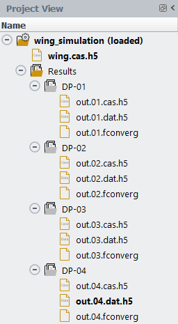
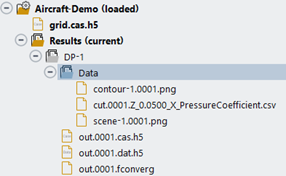
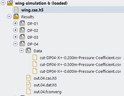
Once a Fluent Aero simulation is complete, clicking the Project View will now display a Results folder inside the Simulation folder. The Results folder will contain subfolders corresponding to each simulated design point, and each of these subfolders will contain associated case (.cas[.h5]), data (.dat[.h5]) and convergence (.fconverg) files. The .fconverg file contains the output of the residuals and monitors and is used to create the Convergence plots. A Data folder appears inside the design point folder when some comma separated value files or image files are saved.
The image below shows an example of a Results folder.