


Two files are used to store the simulation and design point settings; the run.settings file and the projectname.flprj. The following section describes the breakdown of which settings that are included in each file.
run.settings File Stored Settings
Inside the Results folder of every Fluent Aero simulation is a run.settings file that contains settings related to the setup of the boundary zones and the Component Groups step. The run.settings file includes the following settings:
Datamodel settings used by the Geometric Properties, Airflow Physics, Simulation Conditions, Component Groups and Solve steps associated with the Results folder in each simulation.
These settings will be saved to the [projectname].flprj project file when calculating results.
The settings contained in this file will then be used to re-populate the datamodel settings for each of these steps in the Outline View when reconnecting to a previous simulation.
These values will be used by Fluent Aero to check to see if any design points need to be set to when the datamodel step input value has changed.
Datamodel settings used by the Geometric Properties, Simulation Conditions, Component Groups and Solve steps, all table values in the Input: Design Points table, and all table values used to fill the output tables such as the Table:Coefficients and Table:Forces, etc, associated with the Results folder in each simulation.
These settings will be saved to the run.settings file when calculating results.
The settings contained in this file will then be used to re-populate all datamodel settings in the Outline View and all values in the Input: Design Points table when reconnecting to a previous simulation.
The settings contained in this file will also be used to re-populate any relevant metadata in the Project View and projectname.flprj file when reconnecting to a previous simulation.
These values will be used by Fluent Aero to see if any design points needs to be set to when any input parameter have changed.
Notably, if you change the name or type of a zone after have been calculated, the run.settings file will be deleted, and should be re-saved. See Modifying a Zone Type or Name under Modifying Settings After Results Have Been Calculated for more information.
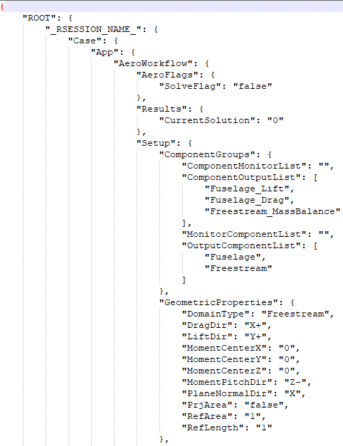
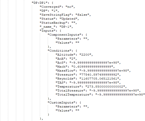
A few portions of an example run.settings file that was opened using a text editor, is shown in the image below. Some relevant information that can be found in the file:
AeroWorkflow:
Contains the settings taken directly from the Datamodel of the Outline View, including the Geometric Properties, Simulation Conditions, and Solve nodes.
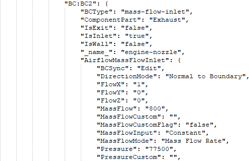
BC:BC#:
Boundary Condition objects which contain settings associated with each Boundary shown in the Component Groups step of the Outline View.
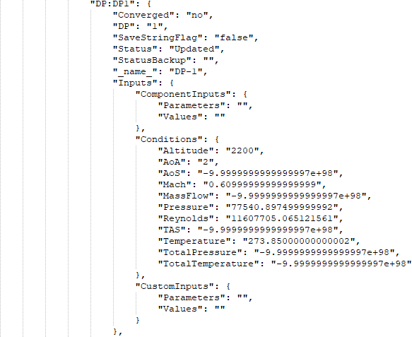
DP:DP#:
Design point objects which contain settings associated with each design point, including their input and output parameters, which are shown in the Input: Design Points table and the output tables such as Table:Coefficients and Table:Forces.
[projectname].flprj file stored settings
Every Fluent Aero project is defined by a project folder [projectname].cffdb, which is a directory that contains all the simulation folders and files, and a project file [projectname].flprj, which is an XML format file that contains information about the files contained in the project folder including their dependencies, location, and additional metadata useful to each item.
Settings contained within the project file metadata can be considered one of the following two types:
Project management settings, such as settings related to the file structure, file dependencies, release information, and historical information, etc., associated with each object.
These settings are solely contained and managed within the [projectname].flprj file.
This information is used to judge file order or connections as necessary when different types of actions are performed, such as post-processing or continuing to calculate, where file dependencies become important.
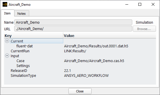
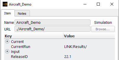
An example of some project management settings associated with a simulation folder called Aircraft_Demo, as shown in the [projectname].flprj file and in the Project View Properties panel, is shown below.
Simulation settings, such as settings related to the simulation and design point conditions, settings, inputs and outputs.
These settings are primarily contained within the run.settings file, but are also shown in the [projectname].flprj file to allow you to easily view these items from the project metadata by selecting the Properties of an item in the Project View.
When reconnecting to a simulation, the run.settings file will be used to overwrite the values in the [projectname].flprj file, so that they are always consistent.
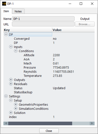
An example of some simulation settings associated with a DP folder called DP-1, as shown in the run.settings file, the [projectname].flprj file and in the Project View Properties panel, is shown below.
Figure 3.11: [projectname].flprj File, Detail Showing Portion of Input Conditions of the DP-1 Folder
![[projectname].flprj File, Detail Showing Portion of Input Conditions of the DP-1 Folder](graphics/g_flu_ug_fluent_aero_post_analysis_dp1_input_conditions.png)
![[projectname].flprj File, Detail Showing Portion of aircraft_demo Simulation Folder](graphics/g_flu_ug_fluent_aero_post_analysis_project_name_flprj.png)
Fluent Aero projects can consume large amounts of disk space, especially for projects with many simulations or design points. Before calculating a simulation, users can selectively disable which files are written using the Files node (refer to Files).
However, to manage the number of files and disk space usage after the simulation has been calculated, it can be helpful to use your operating system’s archiving tools to organize and collect your project files. Some recommendations on how to archive your project and which files can be removed is provided below.
Removing Case and Solution Files from a Fluent Aero Project to Save Disk Space
Design Point Case and Solution Files
When using Fluent Aero with the default Files settings, each design point will save an associated case and data file (out.000#.cas.h5 and out.000#.dat.h5, respectively) written in the simulation’s Results folder. These files typically consume ~90% of the disk space associated with a project, and therefore should be the first files to consider removing if the goal is to reduce disk space.
DP Case Files (out.000#.cas.h5)
These case files contain the complete setup of the design point calculation. This file can be used to calculate the design point results using a separate Fluent Solution Workspace. However, this is NOT required by Fluent Aero to reproduce the results of the design point (Fluent Aero instead uses the run.settings file, along with the top level case file (simname.cas.h5) – which is more space efficient). Therefore, removing all out.000#.cas.h5 files from the simulation Results folders is completely safe and can remove around ~20% of the disk space usage of your project as long the mesh has not been modified.
DP Solution Files (out.000#.dat.h5
These solution files contain the final CFD solutions associated with each design point. They can be used to produce solution contour images, investigate the results, etc. If you only require the post processing information provided in Fluent Aero’s tables (like the aerodynamic coefficients, etc), and do not need to produce any contour images of a design point, you could consider removing these files. However, if you later decide you would like to view the full CFD solution, you would have to recalculate the design point to reproduce the file. Removing all or a majority of these dat files can remove around ~70% of the disk space associated with the project.
Other Files
Fluent Aero can also produce a number of files related to the machine used during simulations or a collection of log files. Some of these files are only required during the calculation and can be safely deleted after the calculation is complete. While it may be helpful to clean up these files for organizational purposes, these file are generally of small size and have negligible contribution to disk space usage. Examples of these files include:
flaero-*.trn, and fluent-*.trn files
These transcript files contain the console log history of the simulations. They can be useful to preserve a detailed history of your calculations. However, they can be deleted if that is not required.
cleanup-fluent-* files
serverinfo-* files
fluent.*.e/o files
job scheduler files
Archiving a Fluent Aero Project using TAR
A complete Fluent Aero project consists of two main files:
a prjname.flprj file, which is an XML format file that contains information about all files associated with the project (location, dependencies, metadata) and,
a prjname.cffdb folder, which contains all the files associated with the project.
These two files should be archived together in a single transportable archive file that can be later unpacked and used.
To archive the entire contents of a Fluent Aero project as one file, the following command can be used:
tar -czvf prjname.tar.gz prjname.flprj prjname.cffdb
It is also possible to exclude certain files (individual, or files that follow a pattern) to archive. For example, if you only want to preserve the simulation setup and tabulated results, you may not want to archive the fluent solution files for each design point. This would reduce the size of the archive considerably. For instance, to exclude all the files that follow the pattern out.*.dat.h5, the following command could be used:
tar -czvf prjname.tar.gz --exclude=out.*.dat.h5 prjname.flprj prjname.cffdb
There are various other options that can be used to exclude certain files, including using a file that lists all files to exclude. Please refer to the documentation associated with your archive tool to learn more.
To later unpack this archive for use, the following command can be used:
tar -xvf prjname.tar.gz
In the Properties panel and metadata of each Fluent Aero simulation, a ReleaseID is stored which shows the release that was used to create the simulation. Furthermore, if a development version was used to create the simulation, a PatchID may also be present.
In the image below, the example simulation was created using the Fluent Aero 2022 R1 release, and therefore, a ReleaseID of 22.1 is shown.
Forward Compatibility Is Not Supported
Fluent Aero simulations are not forward compatible, for example, a Fluent Aero project and a simulation created in a more recent version of Fluent Aero cannot be opened or loaded in an older version of Fluent Aero, as it is possible that the data structure has changed between release versions.
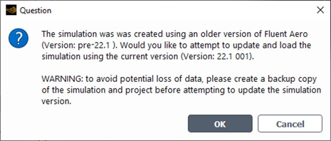
Backward Compatibility: Upgrading and Loading an Old Simulation in a New Release Version
Fluent Aero simulations that were created in a previous version of Fluent Aero may need to be upgraded to support new data structures of new versions. When you try to load a Fluent Aero simulation created in an older release, a window may appear asking if you would like to upgrade the simulation to the new release version.
After the upgrade is complete, the simulation may be used in the new release version. Since unintended changes could take place to a simulation, it is always advisable to first create a backup copy of the simulation files before performing the upgrade.
In situations where a significant version upgrade is not required, a popup may not appear.
When either , , or
is selected, Fluent Aero will enable
species, set the default species model settings in the Solution
workspace and import the air-5species-park93,
air-11species-park93, air-11species-gupta
or mars8species-park mixture. Mixture and species properties
are set by the two-temperature model and can be viewed in the background solver
session, within the Create/Edit Materials dialog under
![]() Setup → Materials after
selecting a mixture in Fluent Aero. In this case, only the material properties of
air-5species-park93 and mars-8species-park
are summarized.
Setup → Materials after
selecting a mixture in Fluent Aero. In this case, only the material properties of
air-5species-park93 and mars-8species-park
are summarized.
Properties of air-5species-park93 and Its Constituent Species
The following describes the properties of the when the Two Temperature model is . See Figure 3.13: Mixture Properties for air-5species-park93 with the Two-Temperature Model Enabled
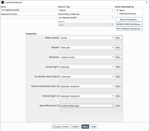
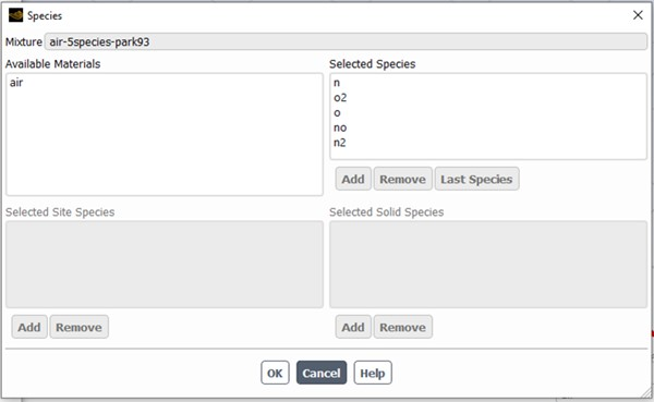
The mixture contains 5 fluid-phase species: atomic-nitrogen (n), oxygen (o2), atomic-oxygen (o), nitrogen-oxide (no) and nitrogen (n2), as shown in Figure 3.14: Constituent Species of air-5species-park93. The properties of each species are shown in these figures:
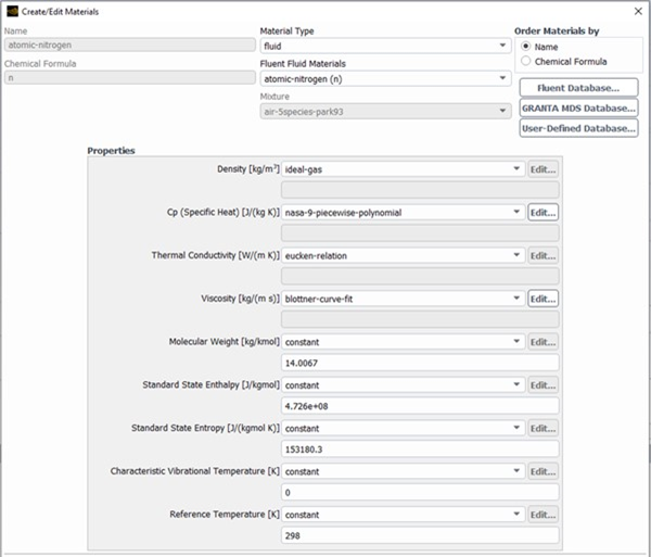
Figure 3.15: Species Properties of Atomic-Nitrogen (n) Set by the Two-Temperature Model
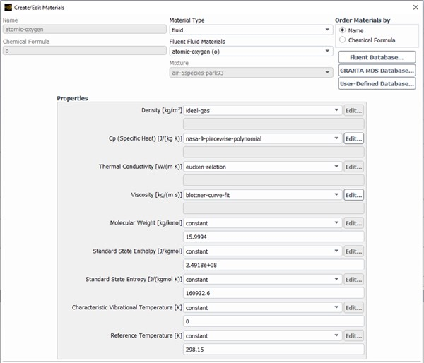
Figure 3.16: Species Properties of Atomic-Oxygen (o) Set by the Two-Temperature Model
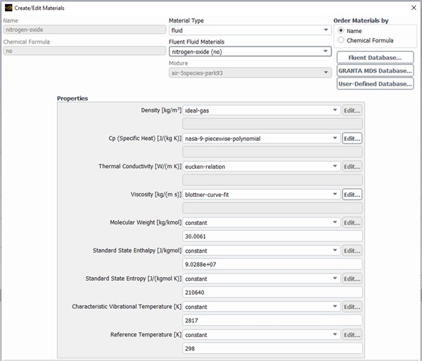
Figure 3.17: Species Properties of Nitrogen-Oxide (no) Set by the Two-Temperature Model
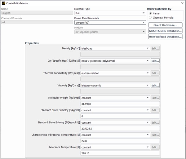
Figure 3.18: Species Properties of Oxygen (o2) Set by the Two-Temperature Model
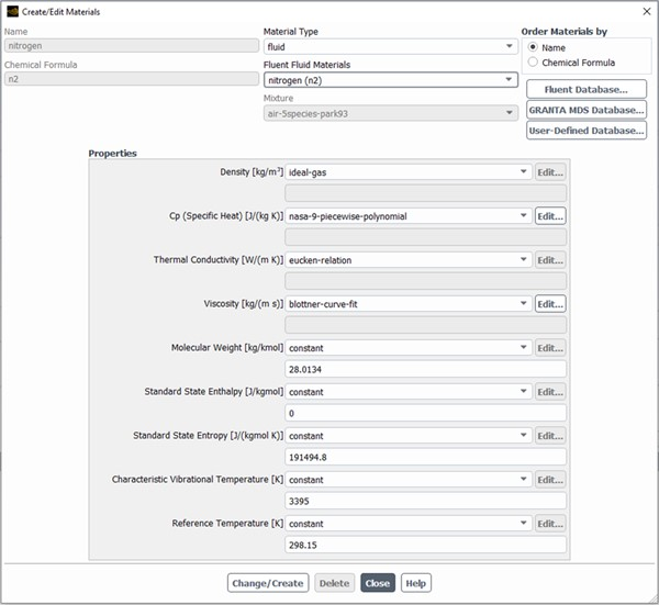
Figure 3.19: Species Properties of Nitrogen (n2) Set by the Two-Temperature Model
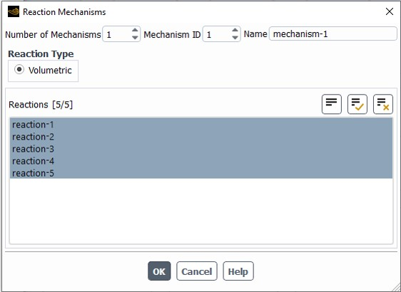
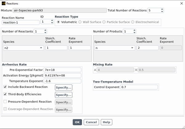
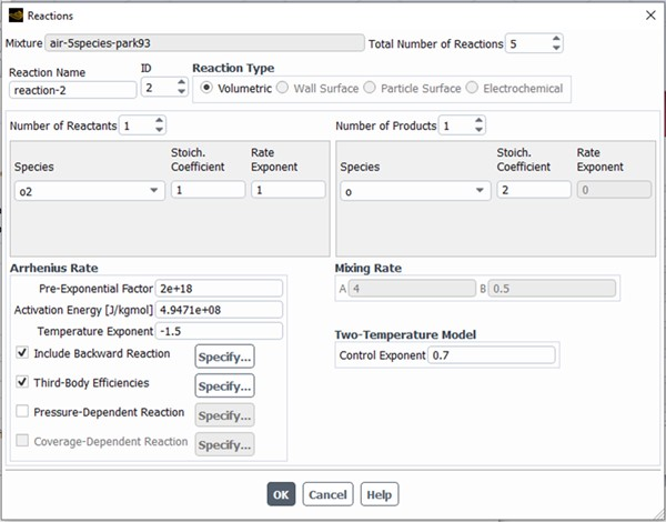
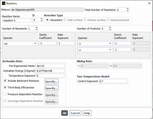
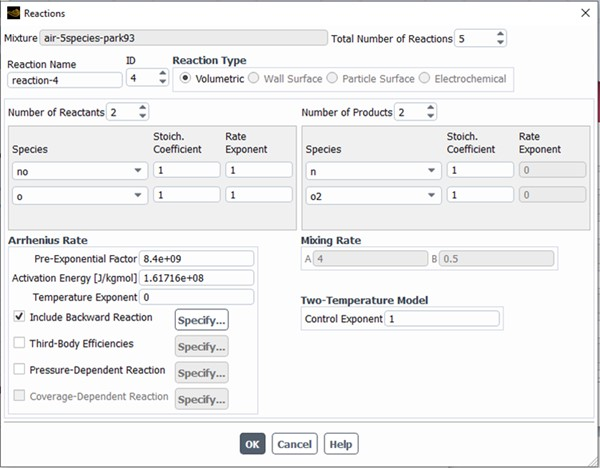
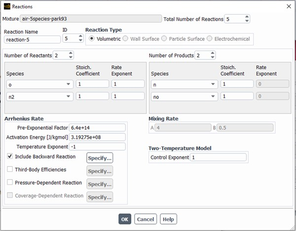
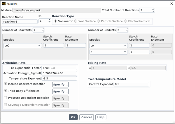
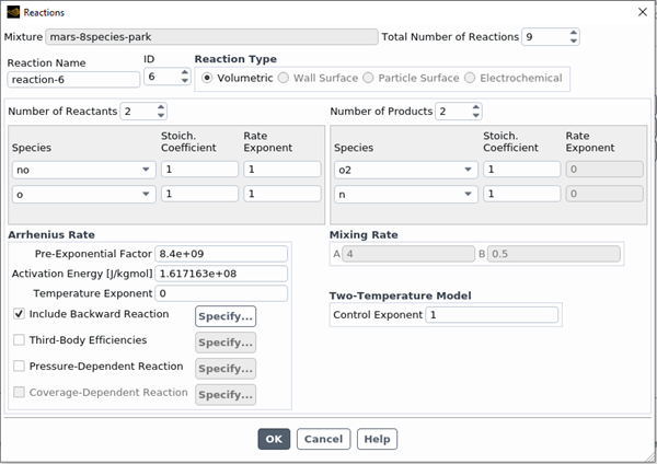
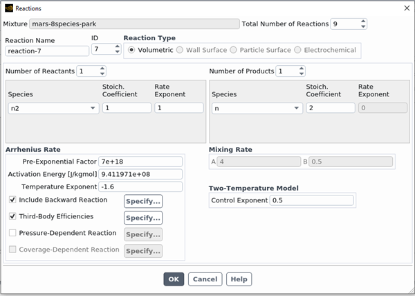
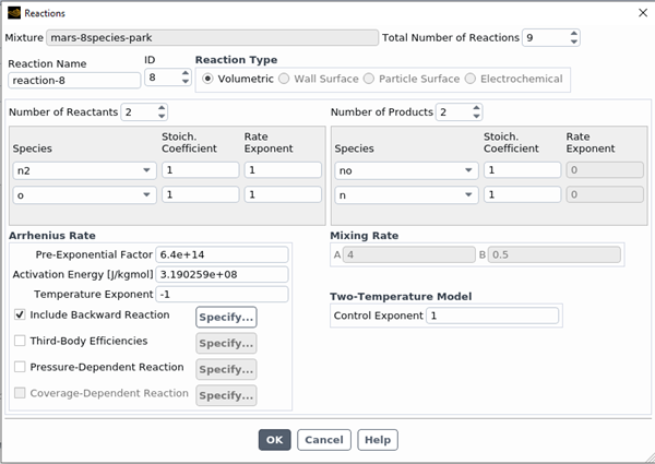
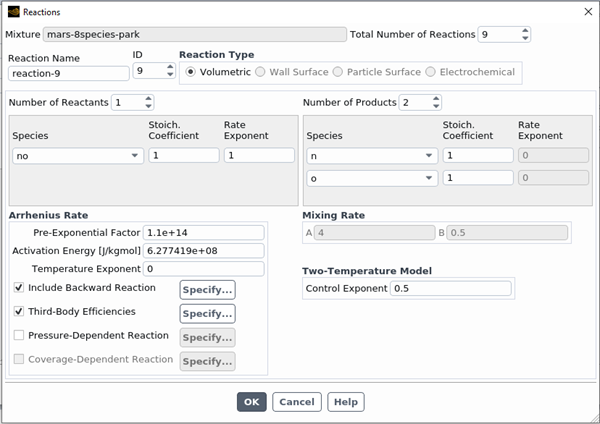
Reaction Mechanisms
The default reaction mechanisms of the mixture are used by Fluent Aero. These are shown in:
Properties of mars-8species-park and Its Constituent Species
The following describes the properties of the when the Two Temperature model is , Figure 3.26: Mixture Properties for mars-8species-park with the Two-Temperature Model Enabled.
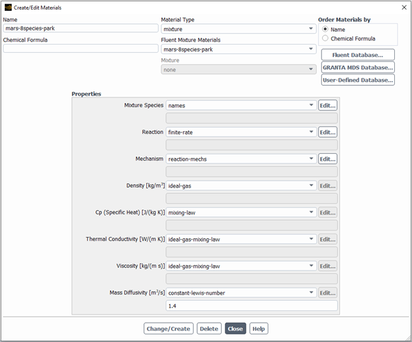
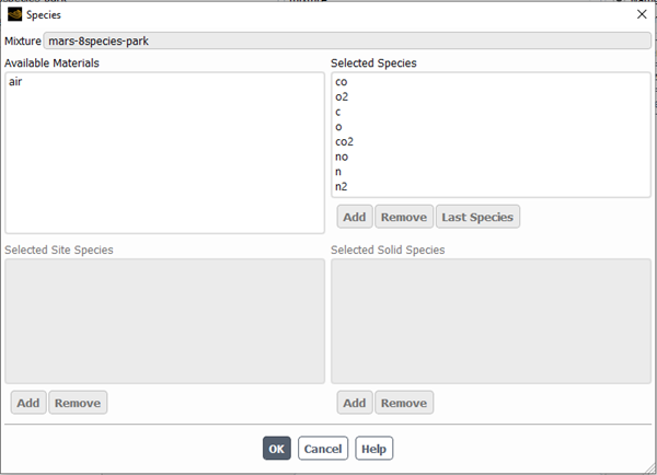
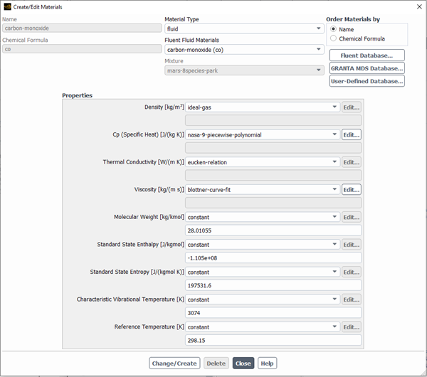
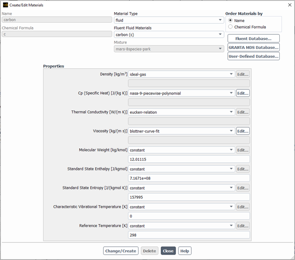
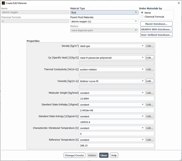
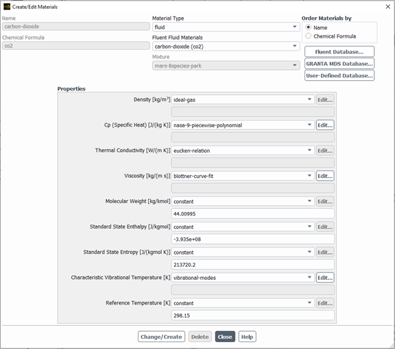
The mixture contains 8 fluid-phase species: (co), (o2), (c), (o), (co2), (no), (n) and (n2), as shown in Figure 3.27: Constituent Species of mars-8species-park. The properties of each species imposed by the two-temperature model are shown in the following figures:
Figure 3.28: Species Properties of Carbon-Monoxide (co) Set by the Two-Temperature Model
Figure 3.30: Species Properties of Oxygen (o2) Set by the Two-Temperature Model
Figure 3.29: Species Properties of Carbon (c) Set by the Two-Temperature Model
Figure 3.31: Species Properties of Atomic-Oxygen (o) Set by the Two-Temperature Model
Figure 3.32: Species Properties of Carbon-Dioxide (co2) Set by the Two-Temperature Model
Figure 3.33: Species Properties of Nitrogen-Oxide (no) Set by the Two-Temperature Model
Figure 3.34: Species Properties of Atomic-Nitrogen (n) Set by the Two-Temperature Model
Figure 3.35: Species Properties of Nitrogen (n2) Set by the Two-Temperature Model


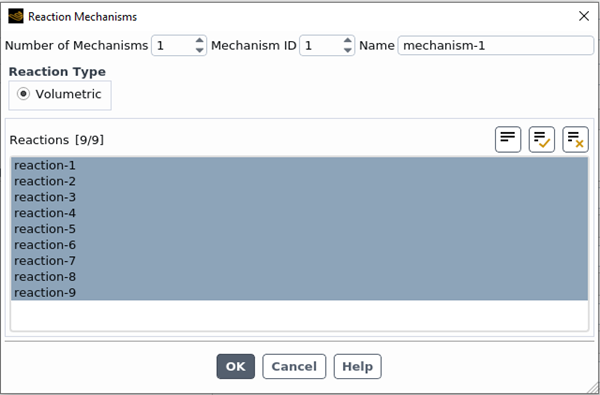
Reaction Mechanisms
The default reaction mechanisms of the mixture are used by Fluent Aero. These are shown in:

Save Image
Enable to save the current result image when executing the Save Current DP Images or Save All DPs Images command.
X [m]
Specify the x-component of the point location.
Y [m]
Specify the y-component of the point location.
Z [m]
Specify the z-component of the point location.
Allows you to create a new, or edit existing line surfaces.
Save Image
Enable to save the current result image when executing the Save Current DP Images or Save All DPs Images command.
First Point
X [m]
Specify the x-component of the first point of the line.
Y [m]
Specify the y-component of the first point of the line.
Z [m]
Specify the z-component of the first point of the line.
Second Point
X [m]
Specify the x-component of the second point of the line.
Y [m]
Specify the y-component of the second point of the line.
Z [m]
Specify the z-component of the second point of the line.
Allows you to create a new, or edit existing rake surfaces.
Save Image
Enable to save the current result image when executing the Save Current DP Images or Save All DPs Images command.
Number of Points
Specify the number of points to have as part of the rake surface.
Start Point
X [m]
Specify the x-coordinate of the starting point of the rake surface.
Y [m]
Specify the y-coordinate of the starting point of the rake surface.
Z [m]
Specify the z-coordinate of the starting point of the rake surface.
End Point
X [m]
Specify the x-coordinate of the ending point of the rake surface.
Y [m]
Specify the y-coordinate of the ending point of the rake surface.
Z [m]
Specify the z-coordinate of the ending point of the rake surface.
Allows you to create a new, or edit existing plane surfaces.
Save Image
Enable to save the current result image when executing the Save Current DP Images or Save All DPs Images command.
Creation Mode
Choose how the plane should be created. A plane can be created using Three Points, using a Point and Normal vector, or by specifying the XY, YZ, or ZX planes.
Bounded
Select to have your plane bounded by the extents of the domain.
X [m]
Specify the x-coordinate of the point in the plane creation.
Y [m]
Specify the y-coordinate of the point in the plane creation.
Z [m]
Specify the z-coordinate of the point in the plane creation.
Point 0
x0 [m]
Specify the x-coordinate of the first point in the plane creation.
y0 [m]
Specify the y-coordinate of the first point in the plane creation.
z0 [m]
Specify the z-coordinate of the first point in the plane creation.
Point 1
x1 [m]
Specify the x-coordinate of the second point in the plane creation.
y1 [m]
Specify the y-coordinate of the second point in the plane creation.
z1 [m]
Specify the z-coordinate of the second point in the plane creation.
Point 2
x2 [m]
Specify the x-coordinate of the third point in the plane creation.
y2[m]
Specify the y-coordinate of the third point in the plane creation.
z2 [m]
Specify the z-coordinate of the third point in the plane creation.
Normal
ix
Specify the x-component of the vector in the plane creation.
iy
Specify the y-component of the vector in the plane creation.
iz
Specify the z-component of the vector in the plane creation.
Allows you to create a new, or edit existing iso-surfaces.
Save Image
Enable to save the current result image when executing the Save Current DP Images or Save All DPs Images command.
Field
Select the field variable that you want to use for creating the iso-surface.
Iso-Value
Specify a value to apply to the iso-surface.
Minimum
The minimum value of the selected field.
Maximum
The maximum value of the selected field.
Restrict to Specific Surfaces
Select to restrict the iso-surface to a particular surface.
Surfaces
Select the surface(s) that you want to restrict to the iso-surface.
Restrict to Specific Zones
Select to restrict the iso-surface to a particular zone.
Zones
Select the zone(s) that you want to restrict to the iso-surface.
Allows you to create new, or edit existing mesh objects.
Name
Define the name of your mesh plot.
Shrink Factor
Specify a value for the mesh shrink factor. To distinguish individual faces or cells in the display, enlarge the space between adjacent faces or cells by increasing this value.
Surfaces
Select the surface(s) where you want to display the mesh.
View
This option allows you to specify an existing view for displaying the mesh. If the current mesh is visible in the graphic window, you can also save the adjusted view by right-clicking on the mesh object and choosing the SaveView command. The View will then be updated and saved as aero-view-<mesh-graphic-object-name>.
Save Image
Enable to save the current mesh image when executing the Save Current DP Images or Save All DPs Images command.
Options
Nodes
Select to include nodes in the mesh display.
Edges
Select to include edges in the mesh display.
Faces
Select to include faces in the mesh display.
Edge Options
Type
Choose how the edges will be displayed, all edges, edges within a specific feature angle, or just the outline.
Feature Angle
Specify a value for the edge feature angle to control how you can display certain features in complex geometries.
Coloring
Automatic
Select to use automatic mesh coloring, where the coloring is automatically determined by either boundary type or ID. If disabled, you can color faces, edge, and node independently.
Color By
Specify whether to automatically color the mesh by boundary type or by boundary
ID.
Color Faces By
Specify a color to apply to faces.
Color Edges By
Specify a color to apply to edges.
Color Nodes By
Specify a color to apply to nodes.
Allows you to create new, or edit existing contour objects.
Name
Define the name of your contour plot.
Field
Select the field variable that you want to use for creating the contour plot.
Surfaces
Select the surface(s) where you want to display the contour plot.
Use Node Values
Select to use values that have been interpolated to the nodes, or computed cell-center values in the contour plot.
Use Boundary Values
Enabling Use Boundary Values in addition to Use Node Values, displays interpolated boundary face values, when available. If Use Boundary Values are enabled with Use Node Values disabled, then the displayed values are boundary face values (not interpolated), if available.
Display Filled Contour
Select to visualize the contour plot using filled contours.
Contour Lines
Select to visualize the contour plot using just contour lines.
Coloring
Choose whether you want a smooth, transitional display of contours or a delineated, banded display of contours.
Draw Mesh
Enable to draw the mesh with the contours.
View
This option allows you to specify an existing view for displaying the contour. If the current contour is visible in the graphic window, you can also save the adjusted view by right-clicking on the contour object and choosing the SaveView command. The View will then be updated and saved as aero-view-<contour-graphic-object-name>.
Save Image
Enable to save the current contour image when executing the Save Current DP Images or Save All DPs Images command.
Range
Auto-Compute Range
Select to automatically determine the range of contour values.
Use Global Range
Select to have the contour display use data from the entire domain.
Clip To Range
Select to have the contour display use data from a specific portion of the domain defined by specified minimum and maximum values.
Minimum Value
Specify a minimum value for the contour data.
Maximum Value
Specify a maximum value for the contour data.
Color Map
Visible
Select to have the color key displayed along with the contour display.
Size
Specify the number of distinct color intervals in the color scale (especially applicable for banded contour displays) or keep the default value. Values from 2 to 100 are acceptable, where increments of 10 are recommended.
Color Map
Select a particular contour color map scheme, or keep the default selection.
Use Log Scale
Select to have the contour display use a logarithmic scale.
Position
Choose the position of the contour color map in the graphics window, or use the default value.
Type
Choose the contour color map presentation of data as general, exponential, or float.
Precision
Specify the numerical precision for the contour color map data.
Automatically Skip Labels
Select to skip a certain number of labels (or show all) in the contour color map.
Skip
Specify the number of color levels to include in the contour color map.
Text Behavior
Specify whether the color map text resizes with the graphics window.
Fixed Font Size
Specify the font size.
Automatic Font Size
Set the initial automatic font size as a ratio of the colormap sub-window for vertically aligned colormaps.
Allows you to create new, or edit existing vector objects.
Name
Define the name of your vector plot.
Vector Field
Select the vector quantity to be plotted.
Field
Select the field variable that you want to use for creating the vector plot.
Surfaces
Select the surface(s) where you want to display the vector plot.
Skip
Specify the number of levels to include in the vector plot.
Style
Select a particular style for your vector markers.
View
This option allows you to specify an existing view for displaying the vector. If the current vector is visible in the graphic window, you can also save the adjusted view by right-clicking on the vector object and choosing the SaveView command. The View will then be updated and saved as aero-view-<vector-graphic-object-name>.
Save Image
Enable to save the current vector image when executing the Save Current DP Images or Save All DPs Images command.
Range
Please refer to the Range section of Contour Properties.
Color Map
Please refer to the Color Map section of Contour Properties.
Vector Options
In Plane
Select to display the vector in the plane normal to the flow.
Fixed Length
Select to have all of the vectors displayed with the same length.
X Component
Select to include the x-component of the vector.
Y Component
Select to include the y-component of the vector.
Z Component
Select to include the z-component of the vector.
Head Scale
Specify a value that can control the size of the arrowhead for the vector display.
Color
Choose a color for the vector arrows.
Scale
Auto Scale
Select to use automatic scaling in the vector display.
Scale
Specify a value in order to increase or decrease the vector scale from the default auto scale value.
Allows you to create new, or edit existing pathlines objects.
Name
Define the name of your pathlines plot.
Steps
Specify the maximum number of steps a particle can advance. A particle will stop when it has traveled this number of steps or when it leaves the domain.
Path Skip
Specify the number of pathlines for better visualization. By default, Path Skip is set to 0, indicating that a pathline will be drawn from each face on the selected surface.
Path Coarsen
Reduce the number of pathlines included in the display.
Color by
Select the field variable to be used to color the pathlines.
Release from Surfaces
Select the surface(s) from which the pathlines will be originating.
View
This option allows you to specify an existing view for displaying the pathlines. If the current pathlines object is visible in the graphic window, you can also save the adjusted view by right-clicking on the pathlines object and choosing the SaveView command. The View will then be updated and saved as aero-view-<pathlines-graphic-object-name>.
Save Image
Enable to save the current pathlines image when executing the Save Current DP Images or Save All DPs Images command.
Options
Oil Flow
Select to display pathlines that are constrained to lie on a particular boundary.
Reverse
Select to reverse the direction of the pathlines display.
Use Node Values
Select to use values that have been interpolated to the nodes, or computed cell center values in the pathlines plot.
Relative Pathlines
Display the pathlines relative to the rotating reference frame.
Range
Auto-Compute Range
Select to automatically determine the range of pathline values.
Minimum Value
Specify a minimum value for the pathline data.
Maximum Value
Specify a maximum value for the pathline data.
Style
Style
Choose from a variety of styles to apply to your pathline display.
Line Width
Specify the width of an individual pathline.
Arrow Space
Specify the space between the line-arrow pathlines.
Arrow Scale
Specify the size of the line-arrow pathlines.
Marker Size
Specify the size of the marker when using marker pathlines.
Diameter
Specify the diameter of the sphere when using sphere pathlines.
Radius
Specify the radius of the sphere when using sphere pathlines.
Width
Specify the thickness of pathlines.
Accuracy Control
Accuracy Control On
Select to mitigate any potential accuracy issues for pathline calculations when using large time step sizes.
Step Size
Specify the steps size used to control accuracy.
Tolerance
Control the error when using large time steps for the calculation.
Color Map
Please refer to the Color Map section of Contour Properties
This section describes the Fluent style Plots. To switch to this style, you need to execute the following python commands in the Fluent Aero console:
Import cx
cx.get("aero-show-plots-advanced")()
Upon execution, the Fluent style Plots will be displayed in the Outline View, as shown in the figure below. If you want to switch back to Fluent Aero style Plots, simply re-execute again the python commands provide above.
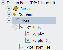
An XY Plot can be used to display the relationship between two variables using data from several surfaces.
To create an XY Plot object, navigate to Results -> Design Point-> Plots -> XY Plots and then click New…. Proceed to the Properties panel of the new XY Plot object as shown in the figure below to define the settings.
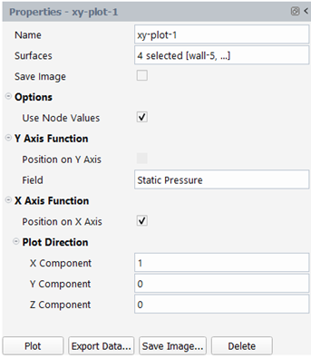
Name
Define a name for the XY plot.
Surfaces
Choose a surface for the XY plot.
Save Image
Enable to save the current plot image when executing the Save Current DP Images or Save All DPs Images command.
Options
Use Node Values
Select to use values that have been interpolated to the nodes, or computed cell-center values in the contour plot.
Y Axis Function
Position On Y Axis
Enable to plot position on the y-axis.
Field
Select the field to plot on the y-axis.
X Axis Function
Position On X Axis
Enable to plot position on the x-axis.
Plot Direction
X Component
Specify the x-component of the plot direction.
Y Component
Specify the y-component of the plot direction.
Z Component
Specify the z-component of the plot direction.
The commands available include Plot, ExportData, SaveImage…, Delete and Copy…. The last three commands are the save as described in the beginning of section Design Point.
Plot
This command allows you to plot the xy plot in the Graphics window.
Export Data
This command allows you to export the data of your xy plot.
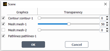
Allows you to create new, or edit existing scene objects.
Name
Define the name of your scene plot.
Graphics Objects
Select the graphics objects to include in the scene. You can also adjust the transparency of contour and mesh objects.
View
This option allows you to specify an existing view for displaying the scene. If the current scene object is visible in the graphic window, you can also save the adjusted view by right-clicking on the scene object and choosing the SaveView command. The View will then be updated and saved as aero-view-<scene-graphic-object-name>.
Save Image
Enable to save the current scene image when executing the Save Current DP Images or Save All DPs Images command.
Scene Colormaps
Once the scene is displayed, you can move the colormaps by left-click and drag. Colormaps can also be resized by dragging the corners of the box that appears when you hover over the colormap.