


You can set the MPM parameters and select the options that are appropriate for your simulation using the Macroscopic Particle Model dialog box that can be accessed either through the ribbon (as described in Loading the MPM add-on Module) or from the Setup/Models/Macroscopic Particle tree item. From the Macroscopic Particle Model dialog box (Injection tab), you can access the Create/Modify Injection dialog boxes, where you can set the macroscopic particle injection properties (see Specifying Injection Parameters for details).
![]() Setup → Models →
Macroscopic Particle
Setup → Models →
Macroscopic Particle ![]() Edit...
Edit...
The inputs for the MPM are entered using the following tabs:
- Particle Tracking
is where you can define parameters for particle tracking.
- Drag
contains drag law options and parameters for the particle drag calculations.
- Collision
allows you to enable particle-particle and particle-wall collisions and define the collision parameters.
- Deposition
allows you to enable particle deposition on selected surfaces and particles and define the relevant parameters.
- Injections
allows you to define macroscopic particle injections.
- Attraction Forces
is where you can specify parameters for particle-particle and particle-wall attraction forces.
- Initialize MPM
contains controls for initializing the macroscopic particles and displaying particle injections.
Note: The default settings may not be appropriate for your case. You must provide parameter data for your specific material.
For additional information, see the following sections:
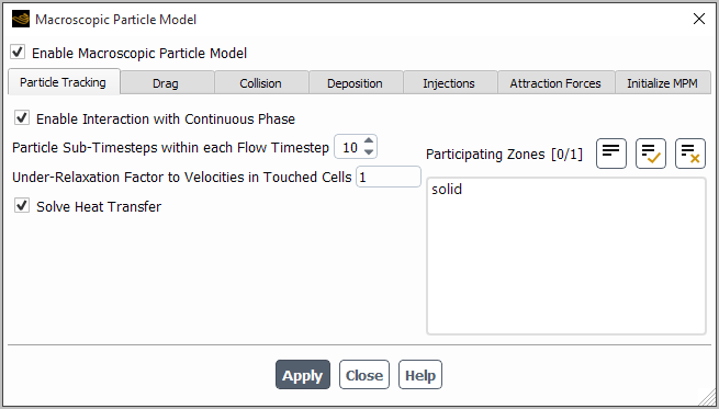
You can use the Particle Tracking tab to control the solution process of the MPM trajectory equations using the following settings (see Figure 25.1: Macroscopic Particle Model Dialog Box (Particle Tracking Tab)):
- Particle Zones
contains a selectable list of the cell zones in which you can use the MPM.
- Enable Interaction with Continuous Phase
(if selected) enables two-way coupling between particles and fluid flow.
- Particle Sub-Timesteps within each Flow Timestep
is a number of sub-time steps for particle tracking in each flow time step.
- Under-Relaxation Factor to Velocities in Touched Cells
By default the under-relaxation factor for fixing velocities is set to
1.- Solve Heat Transfer
enables solving the energy equation. When this option is enabled, you will need to specify Initial Temperature and Specific Heat for a particle material in the Create/Modify Injection dialog box.
Note: The particle time step should be chosen so that macroscopic particles do not cross more than one CFD mesh cell.
Under the Drag tab, you can select an appropriate drag law for your simulation and set the relevant parameters or select Disable Drag Calculations if you do not want to model the drag force in the domain.
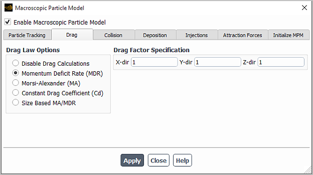
In the Ansys Fluent MPM, the following formulations are available for modeling the drag forces between the continuous and macroscopic particle phases:
Momentum Deficit Rate (MDR) (default)
In this formulation, the momentum exchange coefficient between fluid and solid phases
 is calculated as:
where
 is the drag function, and
  is the macroscopic particle time step size.
The accuracy of the implicit calculations using the Momentum Deficit Rate model depends on number of cells comprising the macroscopic particle. This drag correlation is more suitable for bigger size particles.
Morsi-Alexander (MA)
In the Morsi-Alexander based drag correlation 462 adopted in Ansys Fluent, the Reynolds number for the fluid phase is calculated by:
where,  = fluid density
 = fluid viscosity
 = particle diameter
 = relative velocity of the discrete and fluid phases
The Morsi-Alexander based drag correlation is suitable for smaller size particles.
Constant Drag Coefficient (Cd)
This option implies that the drag is evaluated using a constant drag coefficient. This correlation is suitable for cases where the particle is moving at a certain specified velocity (or acceleration).
Size Based MA/MDR
When this option is selected, the Ansys Fluent solver automatically switches between the Momentum Deficit Rate and Morsi-Alexander drag laws based on a critical diameter. This drag formulation is best suited for cases involving wide range of particle sizes in a single simulation. For particles with a diameter below the value that you specify for Critical Diameter, the Mosi-Alexander drag law will be used. Otherwise, the Momentum Deficit Rate formulation will be used.


You can define a drag factor in a specific direction
(X-dir,Y-dir,Z-dir). A drag
factor of 1 means that the virtual mass force equalizes the momentum difference of fluid in
cells touched by the particle surface within a single flow time step. As a consequence, the
particle sub-time step has to be much smaller (about one-fourth) than the momentum relaxation
time  490:
490:

where  and
and  are the particle and fluid densities, respectively,
  is the particle diameter, and
  is the fluid viscosity.
Besides, the accuracy of the predicted drag depends on the number of cells touched by the particle. At least 20-30 cells are required across the particle diameter.
For multiphase flows, you can select an appropriate fluid velocity field to be used in the drag force calculations. The following options are available in the Multiphase: Drag Based On group box:
Primary Phase Velocity
Secondary Phase Velocity
Volume-Weighted Mixture Velocity
The Collision tab allows you to model the effects of particle-particle and particle-wall collisions.
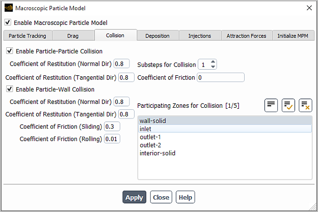
To account for collisions between particles:
Select Enable Particle-Particle Collision.
Specify the following parameters:
- Coefficient of Restitution (Normal Dir)
corresponds to
 in Equation 13–6.
- Coefficient of Restitution (Tangential Dir)
corresponds to
 in Equation 13–7.
- Substeps For Collision
is a number of sub-time steps for detecting particle collision in each particle tracking time step.
- Coefficient of Friction
corresponds to
 in Equation 13–8.
If you also want to account for collisions between particles and walls:
Select Enable Particle-Wall Collision.
From the Participating Zones For Collision selection list, select the appropriate walls.
In addition to Coefficient of Restitution (Normal Dir) and Coefficient of Restitution (Tangential Dir) on the selected walls, you can specify the following parameters:
- Coefficient of Friction (Sliding)
corresponds to
 in Equation 13–8.
- Coefficient of Friction (Rolling)
The value for the rolling coefficient of friction will be factored in the friction coefficient
 .
.
You can use the Deposition tab to specify parameters for macroscopic particle deposition and buildup on selected zones.
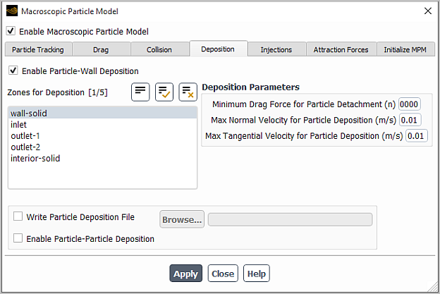
Select Enable Particle-Wall Deposition.
From the Zones for Deposition selection list, select the wall zones on which the macroscopic particles will adhere upon collision.
Specify the following deposition parameters:
- Minimum Drag Force for Particle Detachment
specifies the force at or above which the deposited particles detach from a surface zone.
- Max Normal Velocity for Particle Deposition , Max Tangential Velocity for Particle Deposition
specify the normal and tangential components of the approach velocity at or below which the particles deposit on the surface.
If you want to save particle deposition history data in ASCII format, enable Write Particle Deposition File.
To account for particle agglomeration, select Enable Particle-Particle Deposition. A particle that collides with any previously deposited particles will attach to the particle surface. The deposition parameters that you have specified for particle-wall deposition will be also used for modeling particle-particle deposition.
You can use the Injections tab to create, edit, copy or delete macroscopic particle injections. You can also save all particle injections that you have created to a file for later use or read injections from a previously generated file. The controls under the Injection tab are similar to those found in the Injections dialog box (see Injections Dialog Box in the Fluent User's Guide) with a few minor differences.
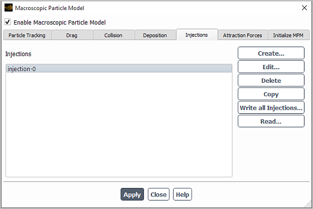
The procedures for creating, modifying and interacting with injections are also similar to those for the DPM injections. The differences related to the MPM injections will be further emphasized. For more information about using these controls, see Creating and Modifying Injections.
To create an MPM injection: click and set the injection properties using the Create/Modify Injection dialog box (see Defining MPM Injection Properties). After the injection is created, it will appear in the Injections selection list, in the Macroscopic Particle Model dialog box.
To edit an existing MPM injection: select it from the Injections selection list, click , and in the Create/Modify Injection dialog box that will open, modify the injection properties as necessary .
To copy an existing MPM injection to a new injection: select it from the Injections selection list and click . The name of the new copied injection appended with
_dwill appear in the Injections list.To delete an existing MPM injection: select it from the Injections selection list and click .
To write information about all injections created in a case: click and in the Select File dialog box that will open, enter the name for the injection file.
Note: Write All Injections... is not supported for steady flows with cemented particles.
To read previously generated injection file into your case: click and in the Select File dialog box that will open, select the injection file to read in. If the injection with the same name already exists in your current case, then Ansys Fluent will rename the imported injection by appending
_dto the name.
You can define the properties of an MPM injection using the Create/Modify Injection dialog box that can be accessed by clicking . The procedure for defining a particle injection is as follows:
(Optional) Change the default name of the injection (
injection-) by entering a new name in the Injection Name entry field.idFrom the Injection Type drop-down list, select the injection type. In the Ansys Fluent MPM, you can create the following types of injections:
point: defines an injection released from a single point.plane: defines uniformly or randomly distributed injections released from a plane.packing: defines an injection of particles packed in a box or cylinder.from-file: allows you to read a text file that defines an injection.
If you want to model fixed particles, enable Cemented Particle(s).
Important: For steady-state simulations, all particles must be cemented.
Specify the particle physical parameters (Diameter and Density).
Note: Note that a material defined in Ansys Fluent cannot be assigned to a particle.
Specify the injection type-specific settings as described in the following sections:
pointinjections: Inputs forpointInjectionsplaneinjections: Inputs forplaneInjectionspackinginjections: Inputs forpackingInjectionsfrom-fileinjections: Inputs forfrom-fileInjections
(Optional) If you want to model a continuous generation of particle injections, select Enable Continuous Injection and in the Define Continuous Injection dialog box that opens when you click Set..., specify the relevant parameters.
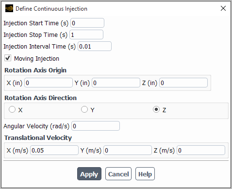
You can specify the following settings:
Injection start, stop, and interval times
New macroscopic particle will be injected into the domain at regular time intervals specified in Injection Interval Time from the Injection Start Time to the Injection Stop Time.
(Optional) Moving and/or rotating injection release point parameters (available when Moving Injection is enabled):
The origin (X, Y, Z) and the direction of the axis (X, Y, or Z) about which the injection is rotating
The Angular Velocity of the injection location
The X, Y, Z components of the Translational Velocity of the injection location
At each time step, the MPM solver determines a new position of a particle injection based on the injection origin at the previous time step and the specified translational velocities.
Click .
The new injection that you have created appears under the Injections selection list.
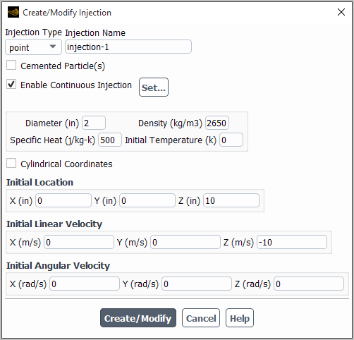
For a point injection of a macroscopic particle, you need to define the following initial conditions in the Create/Modify Injection dialog box:
Particle diameter
Particle density
Specific heat of the particle material (only for heat transfer simulations)
Initial particle temperature (only for heat transfer simulations)
Initial particle release location:
Cartesian coordinates: X, Y, and Z
Cylindrical coordinates: Radius, Angle, and Axial
Particle initial velocity:
Cartesian coordinates: X, Y, and Z
Cylindrical coordinates: Radial, Tangential, and Axial
Particle initial angular velocity
Cylindrical Coordinate System
By default, the global Cartesian coordinate system is used. If you want to specify injection parameters in a local cylindrical coordinate system, enable the Cylindrical Coordinates option, and then define the location of its origin (X, Y, Z) and Axis Direction.
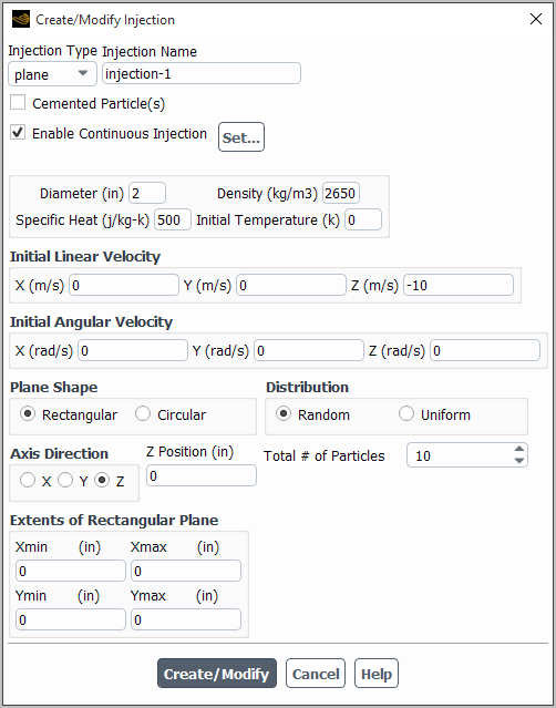
To define macroscopic particle injections released from a plane:
Specify the particle initial conditions as described in Inputs for
pointInjections, except for the particle release location. Note that for plane injections, velocities and initial position can be specified only in Cartesian coordinates.Define the macroscopic particle injection plane.
Two options are available:
Rectangular
Macroscopic particles will be injected from a rectangular plane surface that is offset from a coordinate plane by a distance specified in X, Y, or Z Position in the selected X, Y, or Z axis direction.
The minimum and maximum limits of the rectangular surface are defined under the Extents of Rectangular Plane group box.
Circular
Macroscopic particles will be injected from a circular plane surface that is perpendicular to a selected coordinate direction (X, Y, or Z). The origin and radius of the circle are specified under the Center Location/Radius of Circular Plane group box.
Define the distribution of the particle release locations.
Two modeling options are available:
Random
The MPM will inject particles into a flow domain from random locations on the injection plane. The total number of the released particles is specified in the Total # of Particles integer entry field.
Uniform
The particles will be injected into a flow domain from points arranged in a rectangular pattern. The number of the release points in two axial directions is specified in the appropriate integer entry fields (for example, # of Particles in
X-dir and # of Particles inY-dir).
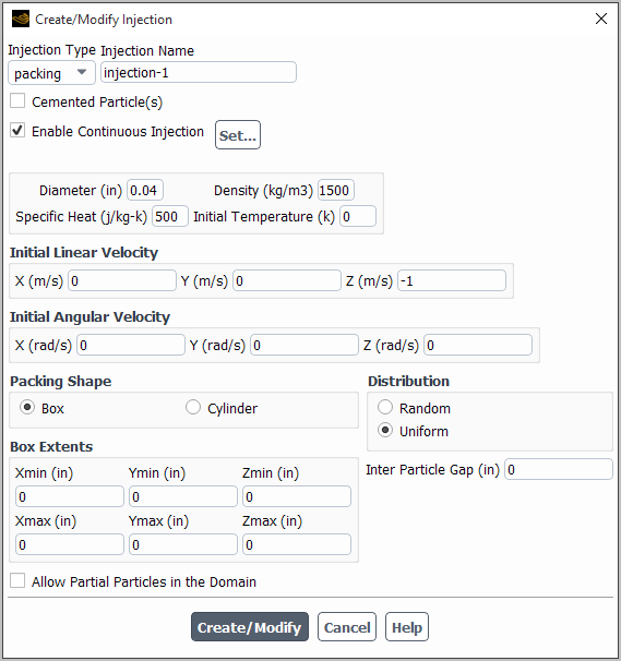
To define an injection of macroscopic particles packed in a box or cylinder:
Specify particle initial conditions as described in Inputs for
pointInjections, except for the particle release location. Note that for plane injections, velocities and initial position can be specified only in Cartesian coordinates.Define the packing region.
For a Box-type packing, specify the minimum and maximum X, Y, and Z coordinates for the packing bounding box under the Box Extents group box.
For a Cylinder-type packing, specify the bounding cylinder axis, minimum and maximum coordinates for the cylinder height, cylinder origin and inner and out diameters.
Define the particle distribution in the packing.
Two modeling options are available:
Random
The initial volume fraction of particles in the packing is specified in the Particle VOF entry field.
Uniform
The distance between particles in the initial spatially uniform packing is specified in the Inter Particle Gap entry field.
If you want to allow a part of the particle to be outside of the domain (with the particle center being in the domain), enable Allow Partial Particles in the Domain.
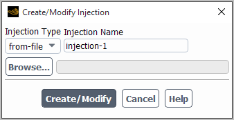
For injections that you want to specify using the from-file option,
the file format is:
number-of-particles
diameter density x-pos y-pos z-pos x-vel y-vel z-vel x-rot y-rot z-rot pstart pstop pinterval cemented
...
where the first line specifies the number of particles
(number-of-particles), followed by
number-of-particles lines that define parameters for the injection
particles. For each particle, you must specify the diameter, density, initial position, linear
and angular velocities, start, end, and interval times, and the integer flag
(cemented in the above file format specification) indicating whether
or not the particle is moving. Note that cemented=1 indicates a
stationary particle, while cemented=0 indicates a moving particle.
Values describing an injection should be separated by one or more spaces and can be specified
using scientific notation (e or E) if needed.
All quantities are in SI units.
An example is shown below:
1
5e-2 5.08e-2 -1e-8 1e-7 2.4e-1 -2e-4 1e-5 1.1 0.0 0.0 0.0 0.0 1e-2 1e-4 0
The Attraction Forces tab allows you to include attraction forces between particles and walls in your problem.
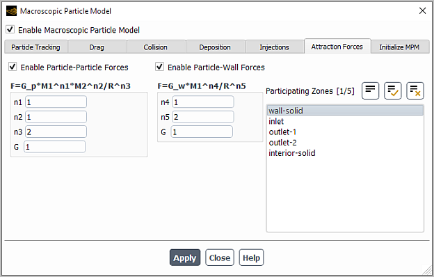
To define the attraction forces between macroscopic particles:
Select Enable Particle-Particle Forces.
Specify the model constants n1, n2, n3, and G_p used in Equation 13–9.
To define the attraction forces between macroscopic particles and walls:
Select Enable Particle-Wall Forces.
From the Participating Zones selection list, select the appropriate zones
Specify the model constants n4, n5, and G_w used in Equation 13–10.
The Initialize MPM tab allows you to apply macroscopic particle related source terms to the continuous phase, initialize macroscopic particles, and display particle trajectories.
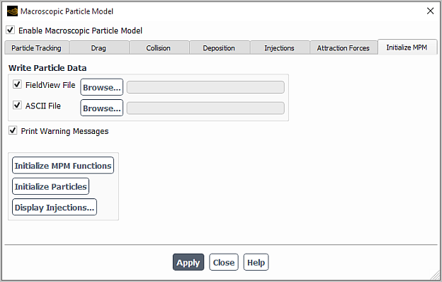
You can also enable the following solution-related options:
Saving particle data in a Field View and/or ASCII format
Printing warning messages related to particle tracking in the Fluent console
Once you have set up the MPM, you need to perform the following steps:
Click .
This will set up macroscopic particle related source terms and apply them to the continuous phase. It will also hook all appropriate UDF functions to the Fluent solver.
Initializing MPM functions adds the following two commands to the solver that will be executed during simulation:
mpm1: displays the particle position(s) at each iteration step.mpm3: writes the particle position(s) at each iteration step in PNG format.
You can disable these commands or modify the reporting frequency in the Execute Command dialog box (accessible from the Solution/Calculation Activities/Execute Commands tree item).
If you want the solver to report or monitor additional solution quantities during calculation, you can define your own execute command(s) using Fluent TUI commands. For more information, see Executing Commands During the Calculation in the Fluent User's Guide.
For coupled simulations, once you click Initialize MPM Functions, the pressure discretization scheme will automatically switch to PRESTO! to provide a more robust solution.
Initialize either the macroscopic particles by clicking or the flow field in the usual way
The macroscopic particle(s) will be introduced into the fluid flow during the next computational time step.
Run the simulation with the injected macroscopic particle(s).
Upon completion of the MPM simulation, you can click Display Injections... and use the Display Particles dialog box to display the computed particle trajectories.
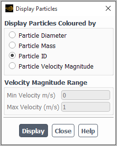
In the Display Particles dialog box, you can select the particle coloring option. You can color particle by the following particle variable values:
diameter
mass
particle ID
velocity magnitude
For the Particle Velocity Magnitude option, you can specify the minimum and maximum range of the velocity magnitude values.