


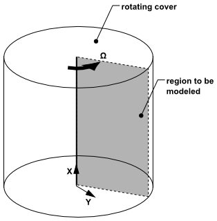
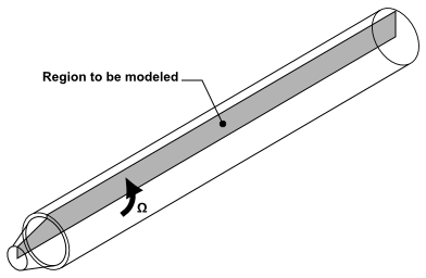
You can solve a 2D axisymmetric problem that includes the prediction of the circumferential or swirl velocity. The assumption of axisymmetry implies that there are no circumferential gradients in the flow, but that there may be nonzero circumferential velocities. Examples of axisymmetric flows involving swirl or rotation are depicted in Figure 1.3: Rotating Flow in a Cavity and Figure 1.4: Swirling Flow in a Gas Burner.
Your problem may be axisymmetric with respect to geometry and flow conditions but still include swirl or rotation. In this case, you can model the flow in 2D (that is, solve the axisymmetric problem) and include the prediction of the circumferential (or swirl) velocity. It is important to note that while the assumption of axisymmetry implies that there are no circumferential gradients in the flow, there may still be nonzero swirl velocities.


When there are geometric changes and/or flow gradients in the circumferential direction, your swirling flow prediction requires a three-dimensional model. If you are planning a 3D Ansys Fluent model that includes swirl or rotation, you should be aware of the setup constraints (Coordinate System Restrictions in the Fluent User's Guide). In addition, you may want to consider simplifications to the problem which might reduce it to an equivalent axisymmetric problem, especially for your initial modeling effort. Because of the complexity of swirling flows, an initial 2D study, in which you can quickly determine the effects of various modeling and design choices, can be very beneficial.
Important: For 3D problems involving swirl or rotation, there are no special inputs required during the problem setup and no special solution procedures. Note, however, that you may want to use the cylindrical coordinate system for defining velocity-inlet boundary condition inputs, as described in Defining the Velocity in the User's Guide. Also, you may find the gradual increase of the rotational speed (set as a wall or inlet boundary condition) helpful during the solution process. For more information, see Improving Solution Stability by Gradually Increasing the Rotational or Swirl Speed in the User's Guide.
If your flow involves a rotating boundary that moves through the fluid (for example, an impeller blade or a grooved or notched surface), you will need to use a moving reference frame to model the problem. Such applications are described in detail in Flow in a Moving Reference Frame. If you have more than one rotating boundary (for example, several impellers in a row), you can use multiple reference frames (described in The Multiple Reference Frame Model) or mixing planes (described in The Mixing Plane Model).