


A FENSAP-TURBO run simulates airflow in a set of turbomachinery components.
The Model panel in the configuration settings of a FENSAP-TURBO run contains the physical models that are going to be used to run a turbomachinery simulation. The Air option in the Physical Model box is set by default.
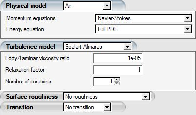
The Continuity and Momentum Equations are used to solve all static components.
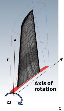
For rotating components, these equations are converted to the relative frame of reference to account for the rotational speed:


where the subscript  refers to the relative frame. The external force vector
 in the momentum equations consist of the Coriolis force,
 , and centrifugal force,
  :
:

where Ω is the rotational velocity of the component and r is the distance from the axis of rotation.
The energy equation for rotating components is:

where  and
and  are the relative internal energy and total enthalpy:

Here  is the relative velocity in the rotating frame, and
 is the tangential velocity of the rotating frame,
  . The Full PDE energy equation is the only
option available in FENSAP-TURBO when solving airflow.
. The Full PDE energy equation is the only
option available in FENSAP-TURBO when solving airflow.
The default turbulence model for airflow simulations in FENSAP-TURBO is Spalart-Allmaras. More details and options for other turbulence models are available in Turbulent Flows.
In this section you will set up airflow options using FENSAP-TURBO.
The Reference conditions in a turbomachine are typically the conditions experienced at the inlet of the first row or freestream, outside the nacelle. The reference conditions in FENSAP-TURBO also establish the reference icing conditions of the first stage. The Conditions panel in the configuration settings is used to establish reference conditions for the airflow simulation.
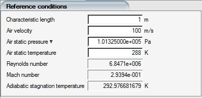
The Characteristic length is typically the span-wise length of a fan or compressor blade or the annular length of a compressor cross-section.
The Air velocity could be either the axial velocity at the inlet of the first row, or the maximum tangential velocity at the tip of the fan blade, a function of the fan speed ω and the tip radius rtip

Air static temperature and Air static pressure are governed by the engine inlet operating conditions. The static pressure and temperature are also used to initialize the computational domain in each component.
At high rotation speeds, or when many stages are present in a single simulation, there is a risk of transient flow reversal at the exits of each stage due to the adverse pressure gradient. To reduce the risk of flow reversal and its impact on convergence, the reference static pressure may be also set to its highest value, static pressure at the exit of the final stage.
Initial conditions set up the initial velocity components for all rows. You may specify Velocity components, Velocity angles or a Solution restart.
specify velocities in X, Y and Z directions.
break up the Reference velocity into X, Y and Z components.
The Solution restart option is used to specify a previous solution file as an initial condition for the present simulation.
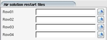
Click the buttons on the right to open the file browser and select the solution file that corresponds to each component.
The list of general boundary conditions is described in Boundary Conditions. The additional conditions required for turbomachinery flows are explained in this section.
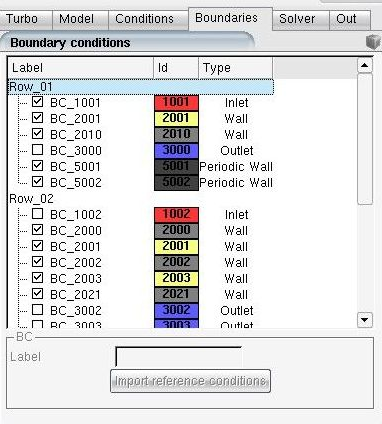
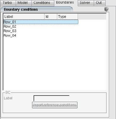
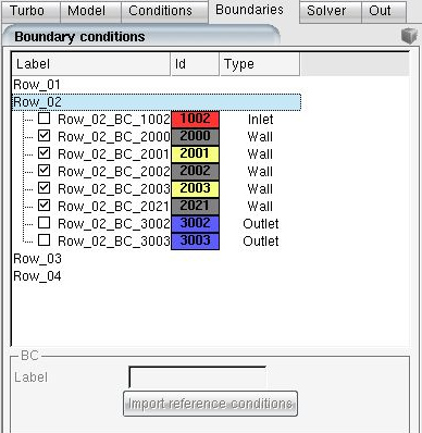
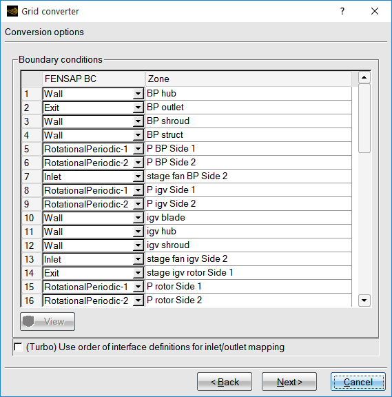
FENSAP-TURBO lists all boundaries present in each sub-component in the Boundaries panel. Boundary condition options for boundaries that are interfaced are grayed out since the boundary conditions are transferred internally.
When many components are present, navigating between components can be challenging. Double-clicking the row maximizes or minimizes the boundaries listed for the row.
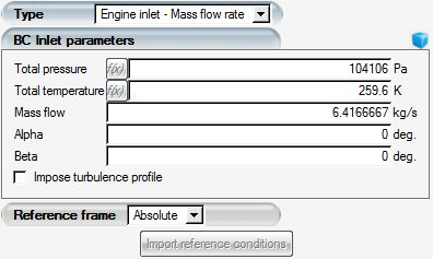
The engine inlet boundary condition can be used for engine intakes to specify Total pressure, Total temperature, and a Mass flow rate. Alternatively if Mach number is known, this value can be set instead of the mass flow rate. It is a 1D-Riemann characteristics based boundary condition that allows a limited variation of the specified total conditions based on flow phenomena that occurs downstream.
This flexibility in allowing small variations of the flow variables makes the boundary condition robust for handling complex flows. It can be used in internal flow applications, such as hot air anti-icing air supply inlets.
Rotating components may contain some wall boundaries that remain static. For example, a fan section, such as the one below, has a rotating blade with a static shroud.
Since FENSAP-TURBO solves rotating components in the relative frame of reference, a counter rotating velocity, equal and opposite to the blades rotational speed must be applied to the shroud wall, and all other components that are static. This condition is applied by selecting the Counter-rotating option from the pull-down menu in the Rotation section.
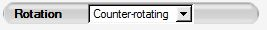
The boundary label turns yellow to identify the wall as a counter-rotating wall boundary. The Counter-rotating option may only be applied to axisymmetric surfaces.
A fluid element subject to forces in the radial direction due to the
tangential (whirl) component of velocity, experiences a pressure gradient in the
radial direction. The pressure gradient  is a function of the radius
  ,
,  and density
  .
.

On outflow boundaries, a radial variation of the static pressure can be imposed by setting the Radial Equilibrium equation option to . For details on how to configure radial equilibrium settings on a subsonic outlet, refer to Subsonic.
Computing EID is a required step to run icing calculations on turbomachinery components. EID runs require adiabatic wall airflow solutions. Refer to Compute EID (Extended Icing Data) for more details.
A turbo solution from CFX can be easily converted to FENSAP-ICE format and set up automatically. Ensure that the following are available in a CFX file before initiating an import:
All reference conditions must be constant values, and not based on expressions. Constant per row rotation values are mandatory. The per row rotation speed must be constant for the solution to be properly converted to the absolute frame of reference. All FENSAP-ICE solutions are read and written in the absolute frame.
CFX solutions with adiabatic walls will need EID calculation by ICE3D before they can be used for icing simulations.
Note: Conditions defined as expressions will be set up with a default value which can be fine-tuned in the import panel in FENSAP-ICE.
In CFX, laminar viscosity and conductivity of air should be set using the icing conditions of your problem. This can be done by adjusting the air material properties within CFX. Otherwise, these parameters will remain at standard atmosphere and will not accurate results.
Start a new project directory or navigate into an existing one.
Start a new FENSAP-TURBO/DROP3D-TURBO run.
Specify the number of rows corresponding to the number of components/zones in the CFX solution file.
Right-click the first grid icon of the turbo configuration and select the Define option. Choose the .res or .def file, and click Next. The following panel will appear:
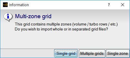
Table 9.2: The Choices Are:
Single grid Will import all the zones in a single grid. Multiple grids Each zone will be imported as a separate grid & solution file. Single zone Used to import a single zone from a CFX file. Note: For turbomachinery runs, the Multiple grids option must be selected. The wall boundaries are automatically identified by FENSAP-ICE and should not need any user intervention.
Click Next to import the solution fields. The flow datafields are automatically assigned based on availability in the .res file.
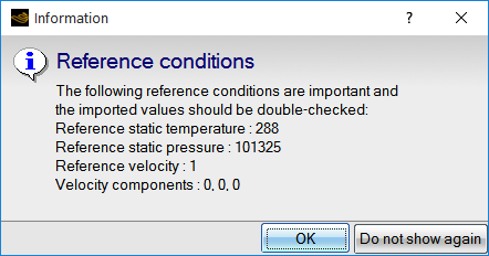
Click Next to assign the reference conditions. Any reference condition that cannot be found in the .res file must be configured manually.
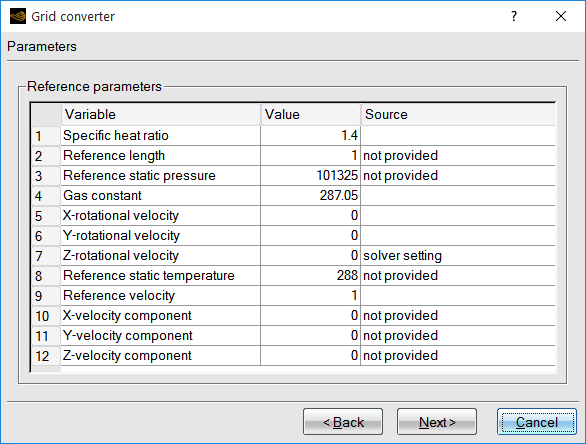
Click Next to finish the grid/solution import process.
Note: If you choose a CFX file that has already been converted, the following message will appear.
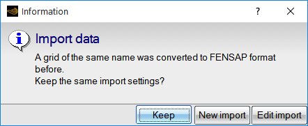
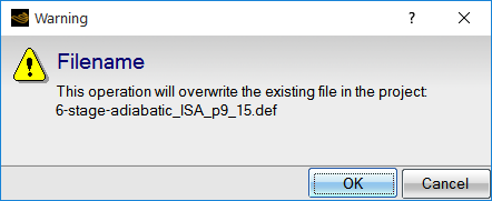
If the same .res file is used to start a DROP3D-TURBO calculation, then select the Keep option. The run will get auto-configured to set up information required to start a turbo calculation. The Edit option allows you to modify boundary condition definitions, reference information imported into a DROP3D-TURBO run. The New import option lets you convert a new grid by overwriting the existing file in the project.
The following options are also available through the command line using the
cfx2fensap command:
Table 9.3: Commands
|
|
|
|
|