


Particle transport equations are hyperbolic and they only need conditions to be defined at upstream boundaries. Inflow nodes are assigned Dirichlet conditions for particle properties, while walls and exits are free. Particles leave the computational domain through walls as water catch and exits. Similar to losing total air pressure through screens, particle concentration is also reduced across these boundaries as a function of the local blockage and water catch on the screens.
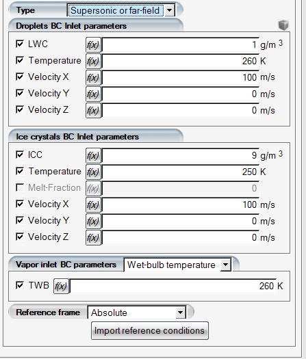
The particle flow boundary conditions are specified only at inlets. The Liquid Water Content or Ice Crystal Content, velocity components and temperature are needed when the Particle thermal equation is enabled (See Particle Thermal Equation).
Melt fraction is available as a boundary condition for crystals when the crystal temperature is 273.15 +- 0.001 K. Crystal species max temperature is currently clipped to 273.15K and any higher value entered as a boundary condition will automatically be clipped within the solver.
When the vapor model is enabled, the vapor amount at the inlet can be specified as vapor concentration, relative humidity, or in terms of wet-bulb temperature.
Each boundary condition can either be constant in space or be a function of the grid coordinates. In this case a formula can be built by clicking the f(x) function button to open the formula window. See Boundary Conditions Varying in Space for an example of how to construct a boundary condition using this feature.
The check marks beside the boundary condition fields serve to allow the solver to use the air flow values or the values found in the particle restart solutions. This is useful when there is a restart file involved and the inflow particle conditions are non-uniform.
Note: For inlet boundaries like engine and nacelle exhausts where the LWC is to be set to 0 kg/m3, particle velocity components can be set equal to the air velocity. This effectively disables the particle momentum equations on these nodes by making the particle relative drag equal to zero and avoids encountering certain numerical issues and convergence problems. To set particle velocities equal to air on such dry inlets, simply uncheck the velocity components.
If there is a droplet or crystal restart file with a non-uniform profile on an inlet that you would like to preserve, uncheck all the variables in the inlet condition panel. This will maintain the restart file state of variables at inlet boundaries.
Click the display icon ![]() to display the boundary velocity vector in the graphical window. Click again to
remove the velocity vector from the graphical window.
to display the boundary velocity vector in the graphical window. Click again to
remove the velocity vector from the graphical window.
For the wall boundary condition, vapor transport modeling provides an option that allows the walls to stay at 100% relative humidity and enables evaporation at these walls. This option is generally not needed in icing related simulations. This model injects vapor into the domain through diffusion from a wall boundary and can be used to track water evaporation from fully wetted surfaces into the surrounding air. Select to activate this wet wall condition.

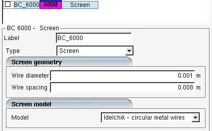
The reduction in liquid water content is simulated by considering the blockage created by the wire mesh. Droplets are collected on the wires, hence the liquid water content past the screen is reduced. In FENSAP-ICE, the droplet collection efficiency of the screen is assumed to be proportional to it’s blockage ratio, which is the area of obstruction, wire cross-sections divided by the total area.
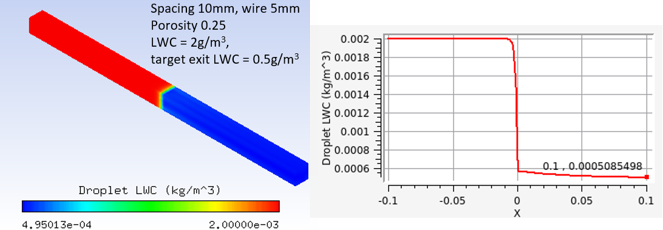
The example below shows a stream of droplets that travel from left to right, passing through a screen (6000) BC with 75% blockage. The initial LWC of 2 g/m3 at the start of the channel reduces to 0.5 g/m3 at the exit plane.
Droplet collection efficiency is computed on the screen facets and used for screen icing calculations in ICE3D to grow the wire thickness.