


FENSAP and DROP3D solve the system of governing equations in non-dimensional form. For this reason, it is important to specify accurate reference conditions.
Important: When performing icing calculations, it is extremely important that all solvers be initialized with the same set of reference conditions. The drag & drop feature of FENSAP-ICE will transfer the reference conditions automatically and is therefore the easiest way to ensure that all solvers are properly initialized.
These reference values are used to transform the Navier-Stokes equations to non-dimensional form.
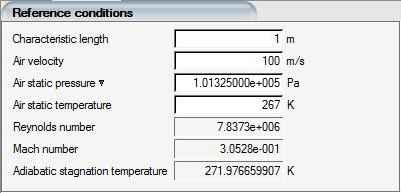
The four reference values to define are:
The characteristic length,

The magnitude of the velocity vector,

The static pressure,

The static temperature,

Other non-dimensional reference variables are automatically computed by FENSAP, such as:
Reynolds number

Reference Mach number

Adiabatic stagnation temperature

The grid coordinates are scaled by the characteristic length.

The fluid properties (laminar viscosity, conductivity, etc.) are initialized using the reference air density, temperature and pressure. The relevant properties are printed in the header of the log file at the start of the execution process.
Note: When carrying out icing simulations with FENSAP-ICE, it is highly recommended that the reference conditions represent the icing cloud conditions and the true air speed (TAS) of the aircraft or test article. In case of helicopter rotor analysis, the blade tip speed is the ideal choice for reference velocity. The reference conditions are used to non-dimensionalize the model equations and the collection efficiency. Certain numerical aspects in DROP3D that are used to improve stability and convergence in the shadow zones will be affected by these settings. Characteristic length should have no impact on the solution other than changing the scale of the residual plots.
Tip: Both Reynolds and Mach numbers should match those of the flight conditions or the experimental data to be compared to. FENSAP computes these two reference quantities and lists them in its Conditions panel and in the log file. It they do not match, the values of the reference pressure, temperature, characteristic length, or the norm of the velocity vector should be adjusted.
The Adiabatic stagnation temperature is particularly useful for glaze ice simulations. In order to obtain meaningful heat fluxes for ICE3D, the temperature that should be imposed on the walls should be a few degrees above this value.
The value of the reference static pressure can be imposed from altitude values according to the US Standard Atmosphere (1976) correlation.
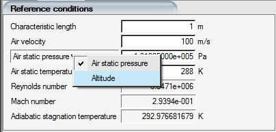
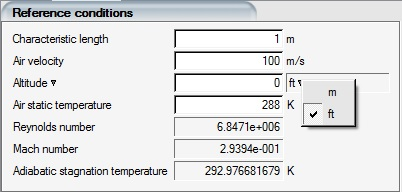
To do so, click the Air static pressure arrow point and select Altitude. FENSAP automatically computes the pressure based on the U.S. Standard Atmosphere (1976). Click again on the Altitude arrow to revert to Air static pressure.
The units for altitude can be changed either to meters or feet by clicking the arrow next to the units.
The Navier-Stokes equations are a non-linear system of equations. The discretized equations are linearized with respect to the primitive variables and then an iterative process is started from an initial guess. If the initial solution is reasonably close to the final one, the iterative process should converge to an accurate solution sooner. For some problems with wide temperature variations (for example a hot jet in cold air), the convergence may be improved by starting the calculation using an initial static temperature more representative of the physics to be solved. To do so, check the box at the bottom of the menu and set the desired initial temperature value.
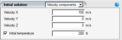
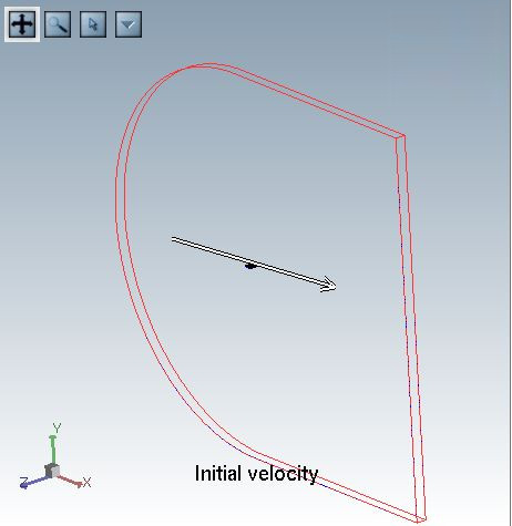
If the option is selected, the three components of the initial velocity vector are imposed throughout the computational domain.
Right-mouse click in any of the three boxes to display a menu that present options to copy velocity values already set during the run configuration process.
If the option is selected, the three components of the initial velocity are obtained from the two angles and the norm of the reference velocity (See Reference Conditions).
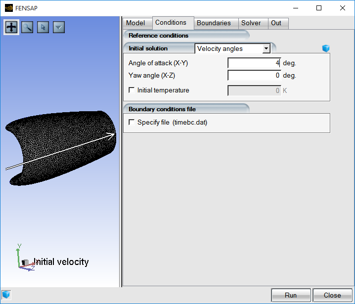
Note: The angle of attack is the angle of the velocity in the X-Y plane. The yaw angle is the angle of the velocity in the X-Z plane. Both angles are in degrees. The exact formula to convert the angles of attack into velocity components and the inverse transformations are:

|

|
where  is the angle of attack (X-Y plane),
  is the Yaw angle (X-Z plane) and
  is the reference air velocity.
If the option Solution restart is selected, the flow field is initialized with a previous flow solution read from a file. This option is used to restart a calculation or to perform calculations at different flow conditions starting from an already converged result.
Note: It is still possible to change the inflow conditions.
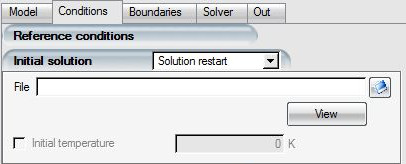
Click the browse button to open the file browser and select the solution file to be used for restarting the calculation.
The restart solution can be post-processed using Fieldview by clicking the button. FENSAP-ICE automatically converts the grid and restart solution file into Fieldview unstructured format and opens the post-processor.
Note: If the grid file is in cylindrical coordinates, the velocity components should be specified as Vr (m/s), Vθ (rad/s) and Vz (m/s).