


In this section you will learn the different capabilities of FENSAP-ICE's native post-processor.
Viewmerical is a simple data post-processor that enables the visualization of FENSAP-ICE grids and solution files. It can be launched from FENSAP-ICE to view most file formats, and can be used in command-line or batch mode. The major features are:
| Features | Action |
|---|---|
|
Grid Display |
|
|
Scalar Solution Display |
|
|
ICE3D Specific Display |
|
|
FENSAP-ICE Specific File Formats (Grids) |
Grids:
|
|
FENSAP-ICE Specific File Formats (Solutions) |
|
The  button in the toolbar permits to launch
Viewmerical:
button in the toolbar permits to launch
Viewmerical:
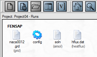
If a grid or solution icon is selected, Viewmerical will be launched to open that file automatically.
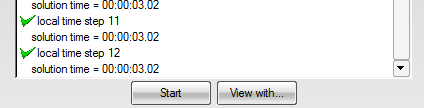
In the solver execution panel, the button will launch the default post-processor.
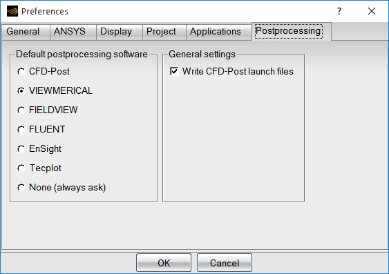
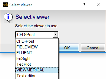
The default post-processor of FENSAP-ICE can be selected in the panel:
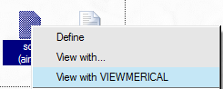
Once configured, the main visualization option in the menus will be Viewmerical. Using the option View with VIEWMERICAL on a solution file will load the selected grid and solution from FENSAP automatically:
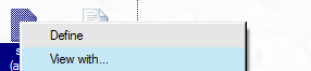
At any time, any alternate post-processor (including Viewmerical) can be launched to view input/output datasets.
Viewmerical can be launched standalone; it does not require a FENSAP-ICE main window or project and can be used on any compatible input file.
Note: A valid FENSAP-ICE license is required to Viewmerical. It can only be used on machines where your license server can be reached. Each license seat of FENSAP-ICE provides a seat for one opened instance of Viewmerical.
The following sections of this chapter are:
Table 16.2: Mouse Control Examples
| Button | Action | +Shift | +Control | +Alt* | Double-click |
|---|---|---|---|---|---|
| Left | Rotation | Zoom | Zoom Box | Pick | Center |
| Right | Zoom/Roll | Menu | |||
| Center | Pan | Center | |||
| Scroll wheel | Zoom |
Tip: Alt button operation might not work in all windowing environments. In such cases, use the toolbar pick icon.
Table 16.3: Controls
| Control | Action |
|---|---|
|
Rotation |
Moving the mouse with the left button pressed will rotate the camera around the object. |
|
Zoom |
Moving the mouse up/down permits to zoom interactively. The scroll-wheel button of the mouse also zooms. |
|
Zoom Box |
With the zoom box selected, moving the mouse left-to-right will permit to draw a zoom rectangle. If the rectangle is drawn right-to-left, the resulting operation will zoom-out. |
|
Zoom/Roll |
In this mode, up-down movements will zoom in-out interactively. Left-right movements will roll around the view axis. |
|
Pan |
Holding the center button (usually the scroll-wheel) and moving the mouse will pan the view. This will move the center of rotation. |
|
Center |
Double-clicking a 3D position to center the display on that point. The center of rotation is moved to the chosen point. |
|
MENU |
See Interactive Menu. |
|
Pick |
Puts you in data query mode (use with the Query panel). |
At the top of the 3D display, a toolbar permits to switch between the main view modes which are normally accessible via mouse + keyboard combinations. See Interactive Menu for the equivalent keyboard/mouse bindings, and the operation description.


Note: Keyboard-mouse combinations described in Mouse Controls will not work if Zoom Box or Pick are enabled. All keyboard-mouse combinations will work correctly if the Rotation mode is selected.

Clicking in the axis window will trigger a view change.
Table 16.5: Axis Display
| Action | Result |
|---|---|
|
Click the X/Y/Z arrows |
Orients the display along that axis. |
|
Click the gray cube |
Orients the display in the default 45 degree isometric view. |
|
Shift + X/Y/Z/gray cube |
Orients the display in the reverse direction (If X-axis would show the front along +X, Shift-click-X-axis would show the back along -X). |
|
Anywhere else |
Keeps the same camera direction; resets the zoom and the center of rotation to view all items. Will use the current Fit to view (visible) or Reset view (domain) settings. |
Right-clicking the axis window provides additional view options:
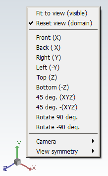
Table 16.6: Additional View Options
| Action | Result |
|---|---|
|
Resets the zoom and center of rotation in order to view all items.
| |
|
Reset the view to this direction. | |
|
Switch between Orthogonal and Perspective. | |
|
Permits to duplicate or repeat symmetric or rotationally periodic datasets. |
A Ctrl left-click in the 3D display, or the usage of the
button  shows the interactive menu:
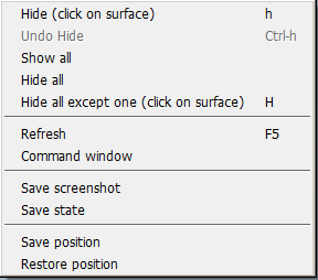
Table 16.7: Interactive Menu
| Menu Item | Result |
|---|---|
| |
|
Undo the previous Hide operation. | |
|
Show/hide all surfaces of all objects. | |
|
All surfaces of all objects are hidden, except the one that was clicked upon. | |
|
Reloads the scalar solution data (if any) from disk. | |
|
Open the 3dview command console window. | |
|
Create a view state file (.views by default) and a command file (.3DCMD by default). If used as command file argument, the command file permits to restart Viewmerical in the saved state. Not all modes and settings are saved. | |
|
Saves a .PNG screenshot to disk. The toolbar and the axis display will not be saved in the image file. | |
|
Viewmerical permits to save the current camera position, and reuse it in later execution. In addition, multiple camera positions can be saved and chosen from.
|
Table 16.8: Keyboard Shortcuts
| Key | Action |
|---|---|
| Backspace | Reset/Fit to view |
| H+click surface | Hide a surface |
| Ctrl+H | Undo the last Hide operation |
| B | Toggle between boundaries display
modes: All, no-SYMM, WALLs only, None |
| U | Undo a view change (rotation/zoom/etc.) |
| Shift+U | Redo a view change removed with U |
| P (hold down) | Pick mode, click an item to select |
| Ctrl+T | Show/Hide the toolbar |
| Space | Show/Hide the right panel (full screen mode) |
| F5 | Refresh - Reload solution from disk |
| 1,2,3,4,5,6,7,8.9.0 | Switch between pre-set views (+X, -X, +Y, -Y, etc.) |
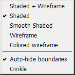
| S | Switch between shading modes |
| X,Y,Z,R,T | Cutting plane mode, if available |
| I | Iso-values mode, if available |
| Up/Down/Left/Right+Shift+Ctrl | Tweak values for the current mode. (Selection of the current
datafield, cutting plane position, number of iso-values
contours, etc.) Left/Right will iterate through numbered datasets, if the step settings are visible in the Data panel |
| Shift+~ | Shows the Viewmerical command line window (See Command Line Usage). |
The following sections of this chapter are:
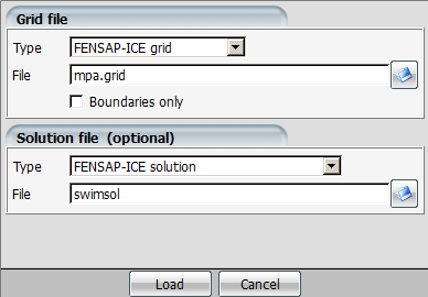
When Viewmerical is launched standalone, or when additional data is to be loaded, this file selection dialog appears:
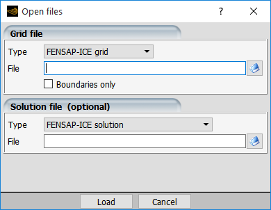
The loaded data can be either grid only or grid and solution.
Table 16.9: Grid File Formats Notes
| Format | Notes |
|---|---|
|
FENSAP-ICE grid |
Grids of the FENSAP/DROP3D/ICE3D file format. Also applies for map.grid and ice.grid. |
|
C3D solid grid |
Grids with material IDs, specific to C3D and CHT3D/solid runs. |
Boundaries Only
Loads only the grid boundaries, not the 3D cells. This will be faster and use less memory. In this mode, it is not possible to display cutting planes or 3D iso surfaces.
Table 16.10: Solution File Notes
| Solution File | Description |
|---|---|
|
|
|
|
|
hflux.dat file output of FENSAP contains facet based data. |
|
|
surface.dat file output of FENSAP contains facet based data. |
|
|
timebc.dat or roughness.dat contains node based boundary condition values. |
|
|
|
| C3D TimeBC |
fluxs1.tot file output of C3D contains facet based data. |
Note: The solution must match the selected input grid.
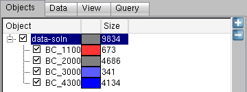
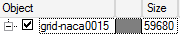
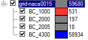
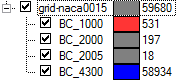
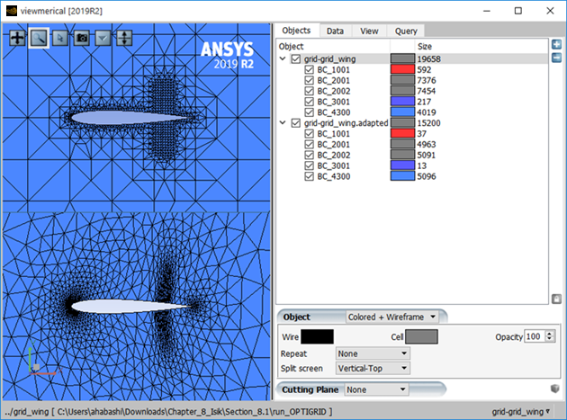
The Objects panel permits to manage the loaded datasets:
 Opens the dialog, to load an
additional Grid/Solution.
Opens the dialog, to load an
additional Grid/Solution.
 Removes the currently selected object.
 Selects all the datasets for modification. (See Lock Selection).
The check box at the left of an object in the object list permits to modify the global visibility of that object.
Regions of a dataset (typically, boundary conditions), can be shown/hidden using the same check box.
Some operations are available or not depending on what the current selection is in the object list.
Object (grid) selected:
Surface (boundary condition) selected:
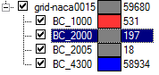
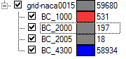
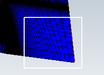
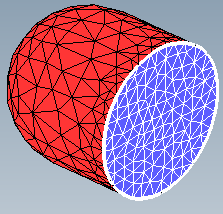
The current selected boundary condition (if any) is shown using a white contour and white wireframe:
In addition to the current selection, multiple selection can be used to perform operations on multiple items in the object list:
Holding down Shift enables adjacent selections from the current item to and including the item clicked.
Holding down Ctrl enables items to be selected and deselected discretely.
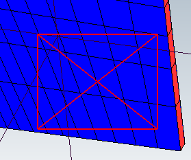
The last item clicked becomes the current selection and, similar to the current selection, is highlighted with a white contour and white wireframe only if it is a boundary condition.
In a single operation, selected items can be modified in the following ways:
Toggling visibility by clicking the item check box.
Changing the shading, color of the wireframe or grid and the opacity in the object dialog.
Enabling and positioning a cutting plane for selected datasets and datasets of selected boundaries.
Modifications on multiple selections that include datasets may affect all boundary conditions of the selected dataset.
The lock selection is used to select all datasets in addition the current item and/or multiple selection items. Operations in a locked selection work similarly to a basic multiple section. This selection can be enabled by clicking the button in the Object Browser (See Adding/Removing Datasets). Locked selection permits similar operations to the shared mode and also enables all data set to the be selected and modified in one operation particularly useful for synchronizing data-field operations or expanding the scope of such operations to include all datasets. The button is in the LUT range dialog (See Shared Range).
This feature is particularly useful when the loaded grids have no associated solution and the LUT range dialog is hidden.
The following sections of this chapter are:
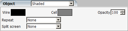
The panel is restricted to color settings should a single surface (boundary condition) be selected in the object list panel:
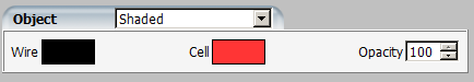
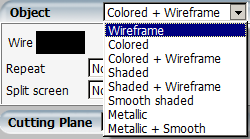
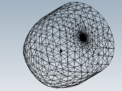
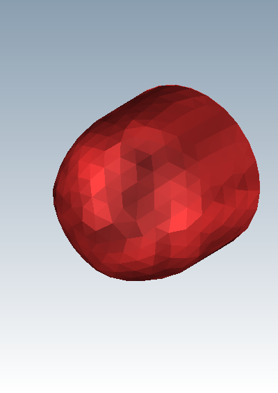
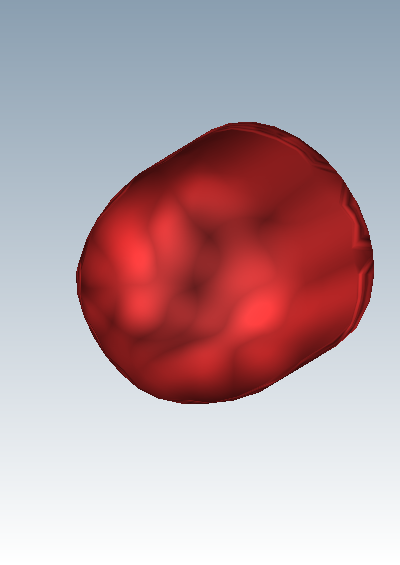
The shading mode is selected at the top of the object panel:

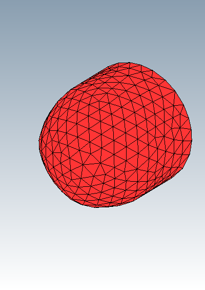


Wire (wireframe lines) and Cell (facets) color can be changed. Click the colored box to access the color picker.
Opacity permits to change the transparency of both wireframe and facets.
Object (grid) selected: The new wire/cell color is applied to all sub-objects.
Surface (boundary condition) selected: The color is applied only to the specified boundary condition.
Note: These settings are useful only for grid types, not colored scalar solutions.
The Repeat options permits to duplicate symmetric data.
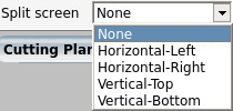
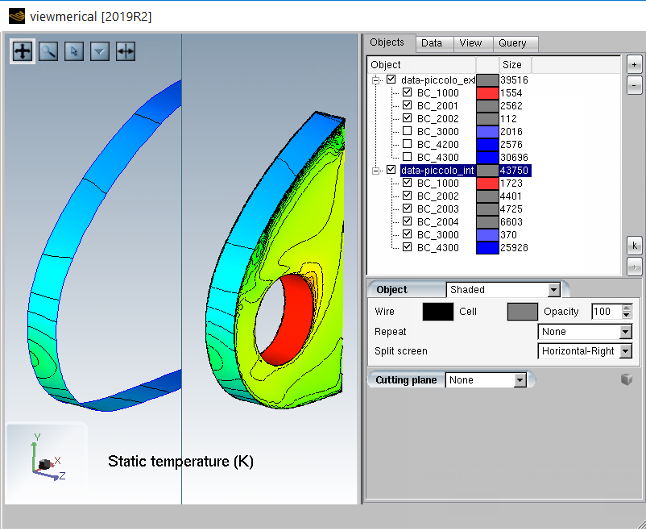
This permits to split the 3D window in two, showing datasets either top/bottom or left/right. The camera position between the two halves is locked, the display are always exactly at the same position.
The split-screen selection applies to the currently selected object, in the Objects list.
Different objects can have different split-screen settings:
To load multiple datasets from FENSAP-ICE:
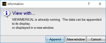
If Viewmerical is already opened with a dataset.
In FENSAP-ICE, load the second dataset using another command. A prompt will then ask you to or open a . Select :
In Viewmerical, select one of the objects in the data list, and choose a Split screen option.
The following sections of this chapter are:
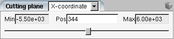
This panel is only available for 3D data. Grids loaded in Boundaries only mode, or 2D data (heat flux, shear stress, timebc) do not offer the cutting plane option.
X/Y/Z-coordinate will select the cutting plane.
Grids providing cylindrical coordinates can also be cut in R or T (Theta).
The slider permits to interactively move the plane between the min and max values.
The minimum and maximum values can be edited, to select a custom range. Entering an empty value (then hitting Enter) will revert to the default range value.
The  icon provides additional display options:
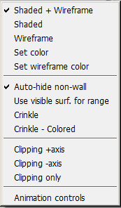
Table 16.11: Display Options
| Menu | Description |
|---|---|
|
, , |
These settings are independent of the individual object/surface settings. |
|
Set color/Set wireframe color |
Changes the colors of the cutting plane elements. |
|
Auto-hide non-wall |
When the cutting plane mode is enabled, all surfaces of the grid are hidden. (Enabled by default). If Auto-hide boundaries are enabled, individual boundary conditions can be shown afterwards using their visibility check box.
|
|
Use visible surf. for range |
By default, the cutting plane range is the full 3D domain of the object (minimum coordinate to maximum coordinate). The range can be restricted to the minimum/maximum of the visible items. For example, if this option is enabled and only the walls are currently visible, the minimum/maximum of the cutting plane zone will be the minimum/maximum of the wall area. |
|
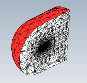
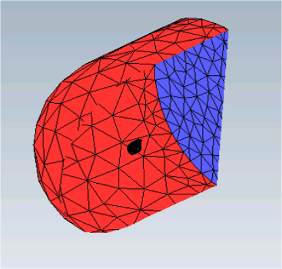
Crinkle |
Instead of displaying the planar intersection of each 3D cell with the cutting plane, the whole cell is displayed. The display is then much cleaner, and the internal 3D topology of the grid easier to visualize.
|
|
|
The crinkle is shaded by element type. Blue = hexa, Green = Prism, Red = Pyramid, White = Tetra. |
|
|
Hide the + or - side of the mesh, in relation to the cutting plane. will hide the cutting plane, while the clipping is enabled.
|
|
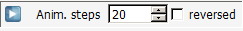
Animation steps |
Displays the animation controls of the cutting plane. Cycling through the domain is controlled by the play/pause button. The step accuracy of the movement and the direction are configurable.
|
The following sections of this chapter are:
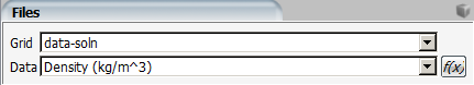
Table 16.12: Files Panel
| Menu Item | Action |
|---|---|
| Grid |
The currently selected dataset. Refer to the Objects panel to add/remove datasets. |
| Data |
If a solution file is loaded, this permits to switch the currently loaded data-field otherwise the data field combo-box is disabled. |
The dataset and data-field are also visible in the combo-boxes at right side the status bar. These combo-boxes can also be used to switch the dataset and data-field:
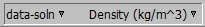
The  button allows you to define an expression for custom fields
using existing fields in the dataset.
button allows you to define an expression for custom fields
using existing fields in the dataset.
The 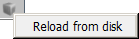 icon offers the option to reload the data from the
disk.
icon offers the option to reload the data from the
disk.
This will reload and display the current dataset, field and step (See Unsteady or Numbered Solutions).
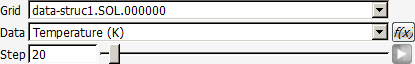
If the loaded solution file is in the format of name.###### (six-digit numbered file) or name.######## (eight-digit numbered file), the Step number, without preceding zeroes, is shown in the panel as well as slider and an button. The slider permits to sweep through the steps, loading/displaying the new solution for each step. The play/pause button triggers a sweep animation for the steps in a continuous loop. If there were initially none included, step animations for the selected datasets are added to the animation item list when an animation is triggered.
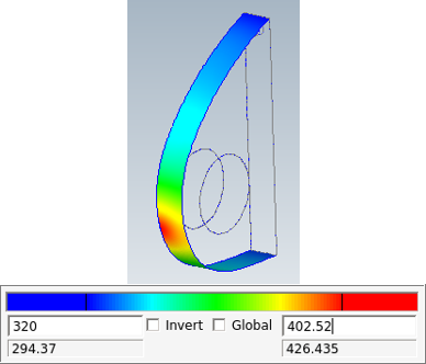
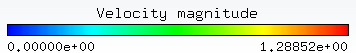
Color Range Panel
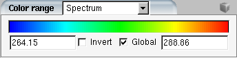
The scalar field loaded is displayed using the settings of this panel. The minimum/maximum values can be edited by modifying the numerical values, or by moving with the mouse the minimum/maximum boundary in the colored box.
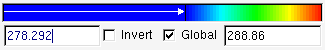
Entering an empty value for the minimum/maximum (with the Enter key), will reset the value to the minimum/maximum value of the dataset (as displayed below).
Invert
Inverts the direction of the spectrum.

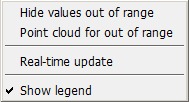
Real-Time Update
Permits to display immediately any change made to the minimum/maximum of the color table.
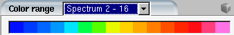
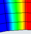
Modes other than Spectrum will use a textured color-mapping table and will permit to have smoother display, but might not be compatible with all 3D display drivers.
Using a color range will give more gradient detail, visible mostly when a facet contains values near the min and the max of the data range.
Spectrum (Linear Interpolation Shading)
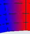
Other colormaps, can show the full gradient of the data:
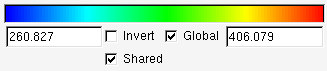
The check box Shared is useful only if multiple solutions of the same type are loaded. Using this option will:
Select the same datafield in all loaded solutions.
Apply any datafield operations to the other loaded solutions.
The global minimum/maximum of all datafields is used for the colormap minimum/maximum.
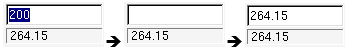
Example 16.1: Multiple Solutions
Solution1 = 260 to 320 K.
Solution2 = 274 to 406 K.
Shared range = 260 to 406 K.
If disabled, the Global setting will use the minimum/maximum only from the visible surfaces.
Default - Global range:
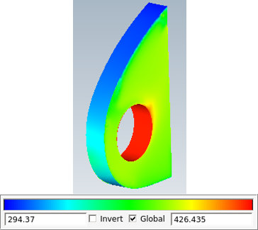
Local data range - With Global check box unchecked and a subset of the surfaces visible:
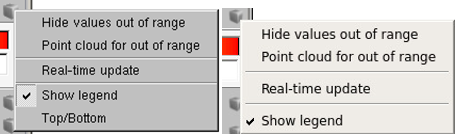
Hide Values out of Range
When a facet has no node within the data range, it will not be drawn (completely invisible).
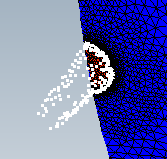
Point Cloud for out of Range
If a node is not in the data range, it is marked with a white point. This option is useful to identify mesh regions where the data is over/under a given threshold.
Important: This option will show a point for each node of the grid, not only surface nodes, this might be many of points to display, if the range is not carefully chosen.
Show Legend
Toggles the display of the legend panel, in the 3D view, for this dataset.
Top/Bottom
Selects the position of the legend panel in the 3D view.
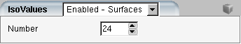
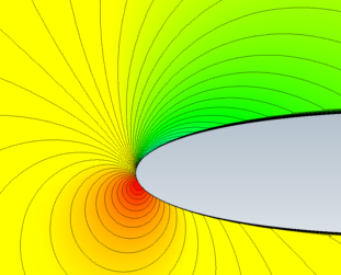
Enabled - Surfaces
This option will display contour lines on the surfaces.
Enabled - Volumes
This option will display 3D Iso-Surfaces.
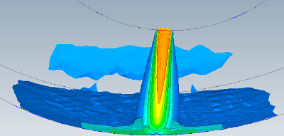
The position of the surface can be adjusted using the color range minimum/maximum values.
Advanced settings are available by clicking the icon:
The options are the same than for the cutting plane (See Cutting Plane Panel).
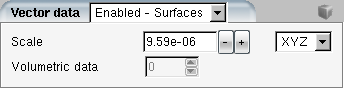
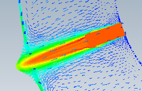
This panel is available only if the loaded solution contains recognized X/Y/Z vector datafields.
| Menu Item | Action |
|---|---|
|
Displays a vector for every visible surface node. | |
|
Displays a vector for a fraction of the volumic nodes. | |
| Volumetric data |
Controls the percentage of volumic nodes to display. |
|
Display a vector for every visible surface node, and for the specified fraction of volumic nodes. |
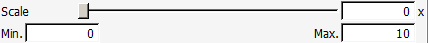
The default vector scale is 1. Meaning that a vector of magnitude 1 will be displayed as size 1 in the scale of the grid. Usually, the vector scale must be changed to be suitable for display, enter a scaling value or use +/- to change it:
Relative and Normalized Scaling
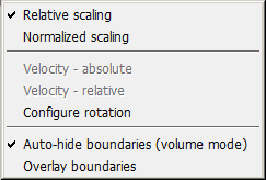
The scaling mode will either display vector with length relative to their magnitude () or all of the same length ():
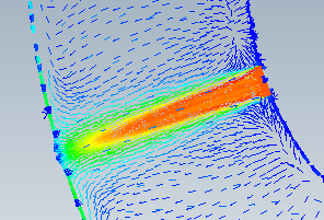

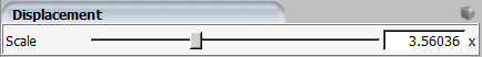
Some data files contains mesh displacement information (such as ALE timebc used for grid displacement). This panel is visible if the Displacement magnitude option is selected. The scaling permits you to deform the grid from the displacement vector. The default range is 0-10 with 0 being the default value:
Enabling the option allows the modifications to be applied immediately to the dataset while moving the slider:
The following sections of this chapter are:
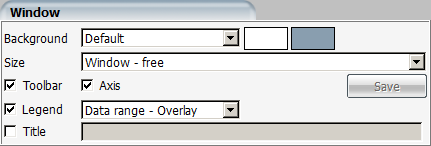
Table 16.13: Window Panel
| Menu Item | Result |
|---|---|
| Background |
Permits to change the background color. |
| Size |
Choose the behavior or resolution for the 3D display viewport or the window size of 3DView. allows the window and viewport be resized freely and is the default option. With a fixed viewport size the window is resizable. With a fixed window size the viewport is resized to fit. Custom sizes can be set using the Width and Height settings for either the viewport of the window. |
| Toolbar/Axis |
Control the visibility of the elements on the screen. |
| Legend |
Selects the mode of display of the dataset legend. |
| Title |
Permits to select a title written at the top of the display, useful for screenshots. |
This mode can be enabled in the Advanced panel (double-click the panel header).
It will render the data for use with red/cyan or red/blue filter 3D glasses:
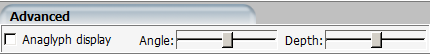
The Angle and Depth settings can be fine-tuned using the sliders.
Grayscale or black & white data is well suited for this type of display.
The following sections of this chapter are:
The currently loaded scalar data-field is used for 2D plots:
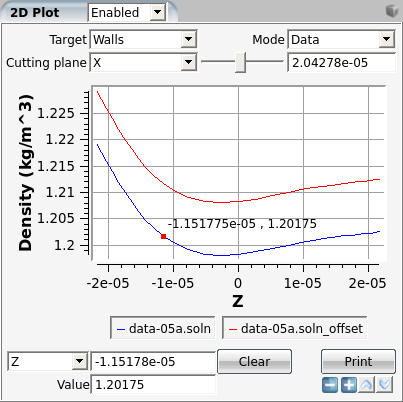
The 2D plot data is computed onto the mesh intersections with a cutting plane.
Table 16.14: Target
| Walls |
| Walls - Visible |
| Inlets |
| Inlets - Visible |
| Outlets |
| Outlets - Visible |
| All items |
| Visible items |
The Target specifies the surfaces onto which the cutting plane will be applied.
To work only on a single wall, on a multi-wall dataset:
Hide all other boundary conditions from the display.
Select or the option of the appropriate target type.
Table 16.15: 2D Window Panel Modes
| Modes | Description |
|---|---|
|
The data-field is evaluated for each intersection point, this value is shown in the Y-axis of the 2D Plot. In Geometry mode, only the grid geometry is used, this is useful to display a iced surface cutting plane maintaining the aspect ratio for the geometry to be plotted. | |
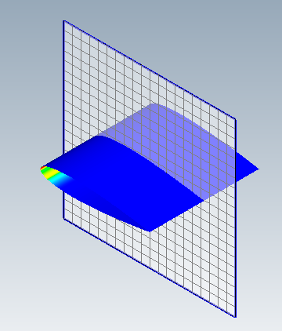
| Cutting plane: |
Specifies the plane and its position. The plane position and alignment is displayed in the 3D window. (The plane is infinite, the displayed grid depends of the visible items bounding box). |
In the plot area:
Left-click will select a point for value query.
Shift drag left button will draw a zoom area, and zoom in.
Dragging the mouse horizontally/vertically will do a horizontal/vertical zoom.
Shift + left-click will zoom-out.
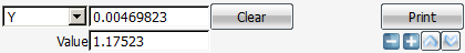
: Selects the coordinate to use for the plot horizontal scale. Distance is the distance from the previous point.
: Send the plot to the default printer.
 : Permits to accumulate multiple plots in the same display.
For example ice cuts at different cutting plane positions, or different icing
time. All the plots must be sharing the same dataset mode (For example, you
cannot mix a temperature plot with a heat flux plot).
: Permits to accumulate multiple plots in the same display.
For example ice cuts at different cutting plane positions, or different icing
time. All the plots must be sharing the same dataset mode (For example, you
cannot mix a temperature plot with a heat flux plot).
: Permits the 2D plot panel to be resized vertically. Horizontal resize is done with the view port and tab splitter grip which affects all the panels.
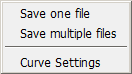
: Save all the date from plot to one plain text file.
: Save data from plot in one plain text file per curve.
: This opens a dialog to edit the width, color and style of visible curves.
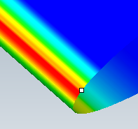
Clicking the 3D data when in picking mode ![]() (Alt + click or P +click)
will select the closest node to the XYZ point clicked upon.
(Alt + click or P +click)
will select the closest node to the XYZ point clicked upon.
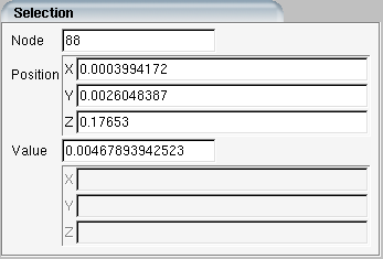
The currently selected node is shown as a white dot:
The node ID is shown in the Node field (node identifiers start at 1).
The node coordinate is in X/Y/Z fields.
The node scalar value, for the currently selected datafield is shown in Value.
If the scalar value is a velocity magnitude, the individual X/Y/Z components are also displayed.
To expand the panel, double-click the Compute header.
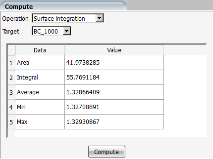
In the Target menu, select the boundary condition to work on and click the button.
Area: Area of the surface boundary condition.
Integral: Integrated value of the current dataset, on the boundary condition.
Average, Min, Max: Statistics of the current dataset, on the boundary condition.
In the Target menu, select the boundary condition to work on and click the button.
This mode is only valid for airflow, and will use the Density and Velocity components of the solution.
Area: Area of the surface boundary condition.
Avg Normal X/Y/Z: Integrated average value of the surface normal.
Integral: Integrated mass flow value.
The following sections of this chapter are:
Viewmerical has a special mode optimized to display ICE3D output files. These output files are:
Table 16.16: ICE3D Output Files
| Output Files | Description |
|---|---|
|
map.grid |
Grid walls on icing surfaces. |
|
ice.grid |
Iced surface (displaced grid of map.grid, with the ice thickness). |
|
swimsol |
Nodal solution, applicable to map.grid/ice.grid. |
The menu/button, from FENSAP-ICE permits to launch Viewmerical in this mode, loading the 3 files automatically. From the dialog, select the FENSAP-ICE grid = map.grid and = swimsol.
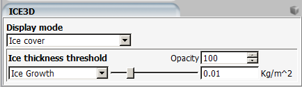
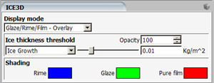
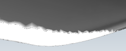
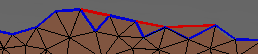
Ice Cover
Displays the ice in white, over a metallic base mesh. The ice is only displayed where the threshold is respected. For example if the ice thickness is more than the specified value. This is used to clip the display of near-zero values. Multiple threshold variables are available.
The default threshold is which is accounting for all the growth since the start of the computation(s). Ice thickness and are based on data relative to the last ICE3D simulation.
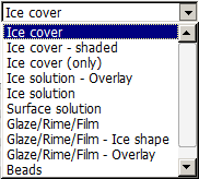
Table 16.17: Display Mode
| Mode | Displays |
|---|---|
|
|
As ice cover, but with some shading on the ice shape. |
|
|
Only displays the ice cover, the shading options and color settings of the current object apply to the ice cover. |
|
|
swimsol scalar data is applied to the ice shape grid (shown with the threshold). |
|
|
swimsol scalar data mapped on the ice.grid shape grid. |
|
|
swimsol scalar data mapped on the map.grid. |
|
|
Displays in colors the zones of Glaze/Rime/Film.
|
|
| CAD Output |
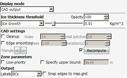
The mode permits to select an iced zone - using the same threshold used for the ice cover display - and save the ice shape to a .stl or point cloud file.
Such files can then be used with CAD or 3D printing software to reconstruct the ICE shape.
From the ice cover:
The surface for the CAD would be:
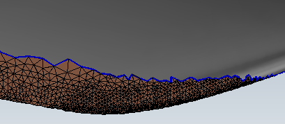
Select the most appropriate threshold, to avoid CAD artifacts.
The surface can be saved to a CAD-friendly file using the options from the gray cube menu.
If the CAD surface contains islands (small surfaces disconnected to the main iced surface), such as:
Or holes in the iced surface:
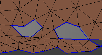
Use the Cleanup options to correct these artifacts.

To remove sharp edges in the CAD boundary, such as:
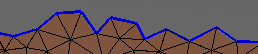
Use the Edge smoothing function:

Additional triangles will be added, to smooth the external edges of the CAD (not present in the original grid, but reusing original node coordinates).
Angle:
More degrees will lead to more smoothing.
Iterations:
Number of times this process is repeated.
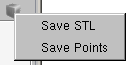
Use the ![]() icon to access the output commands:
icon to access the output commands:
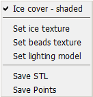
The CAD surface can be exported to a .stl file, readable by most CAD software, or to a point list file.
STL output will write two files: FILE.stl and FILE_surf.stl, FILE.stl is the displaced ice surface, FILE_surf.stl is the base wing surface:

Labels:
For .stl files, from this setting each triangle patch will be saved in a different zone named for each boundary condition (or by Patch/Boundary Conditions+Patches).
Snap edges to map.grid:
In the case of a 3D ice shape (not a 2D periodic/symmetric grid) if the two files are joined together, they can be assembled in a gap-free 3D shape suitable for 3D printing. For a perfectly gap-free shape, Snap edges to map.grid is required, as it will use the coordinates of the wing surface for each of the boundary edges of the iced surface.
Maximum combined cross-section (MCCS) is a method developed at NASA Glenn
Research Center to represent and document ice shapes obtained on 3D swept wings.
These wings accrete ice with scallop and lobster-tail features which are quite
variable in the spanwise direction. Extracting ice shape tracings for 2D data
plotting is not representative of the 3D variations along the span. The
state-of-the-art to document these type of ice shapes include laser scanning the
ice to digitize its shape in STL format. Once available in digital form, several
data cuts perpendicular to the leading edge are done and combined into a single
ice shape curve that traces the silhouette of these cuts. This silhouette is not
the real ice shape, but a combination of all the ice shapes along a section of
the span. Viewmerical does not directly provide a way
to produce the MCCS curve, but it can be used to make such cuts along the span
that can be combined into the MCCS using a python script provided with this
installation package of FENSAP-ICE. The file is located at
fensapice/data/templates/scripts/mccs.py. This script
requires Python version 3 and above, and the libraries
pandas and shapely to be
installed. These libraries are not provided by Ansys but can be downloaded
from their providers. These libraries are available with BSD licenses without
any warranties. You can review each library license disclaimer and terms of use
before using the mccs.py script provided by
Ansys.
The process to use the MCCS script is as follows (Linux):
Install
pandasandshapelyin your local copy of python. This needs to be done only once.In your home directory, create a python environment, and name it
my_venvor another preferred name:python -m venv my_venv
Install the required packages:
./my_venv/bin/pip3 pandas./my_venv/bin/pip3 shapelyLaunching this copy of python will contain the libraries. You can verify by this by running the following:
~/my_venv/bin/python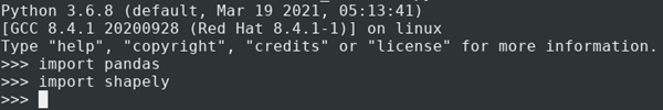
Right-click the config icon of a multi-shot run in the FENSAP-ICE project window and choose to start a Linux command line terminal with FENSAP-ICE environment and paths preset.
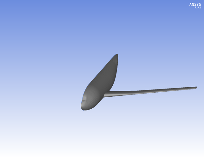
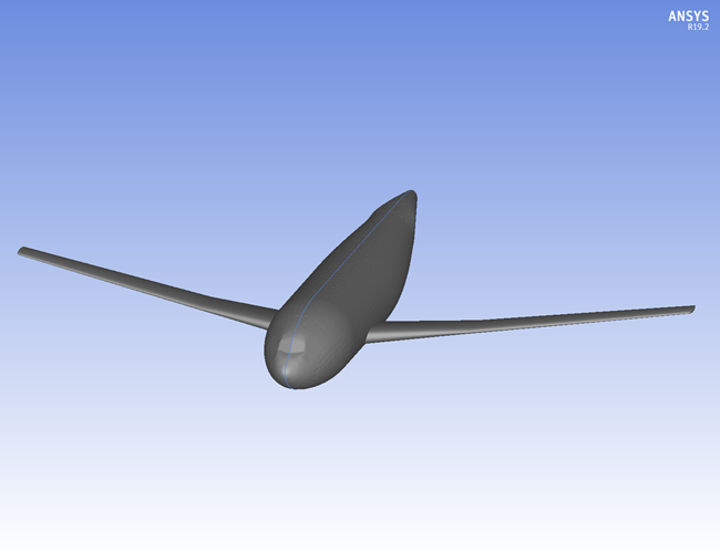
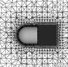
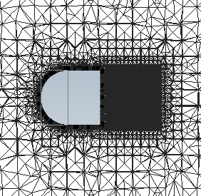
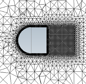
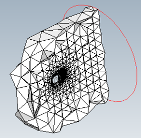
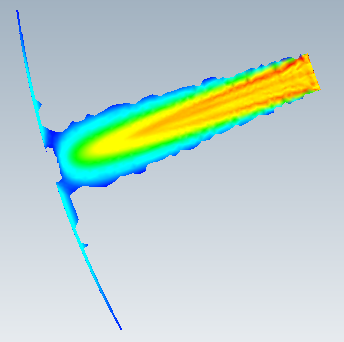
Use the command line tool convertgrid, that should be already accessible with the current path settings, to rotate the iced grid file in the opposite sweep direction to align the leading edge with the span direction main coordinate:
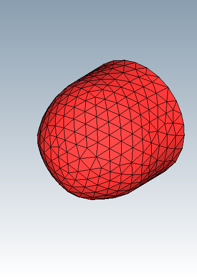
$NTI_PATH/convertgrid ice.grid.ice.000010 ice.grid.rotated
                                -rotateZ=30
Figure 16.20: Shot 10 Ice Grid of a 30-Degree Swept Wing Case Rotated to Align Its Leading Edge With One of the Primary Coordinates (Y in This Case)
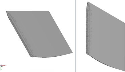
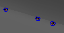
Load the rotated grid file in Viewmerical:
$NTI_PATH/nti_3dview ice.grid.rotatedUsing the Query / function, choose the correct cutting plane direction and save several curves across the span. The
 button at the bottom
right corner of the 2D plot will save a curve. You can drag the graph
panel leftward to increase the length of the slider and have a finer
control on the cut location, or enter the location manually:
button at the bottom
right corner of the 2D plot will save a curve. You can drag the graph
panel leftward to increase the length of the slider and have a finer
control on the cut location, or enter the location manually: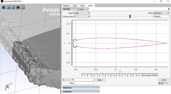
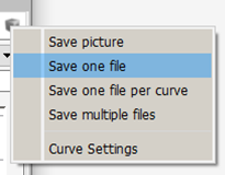
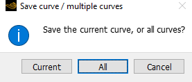
Save all the curves to a single data file using the cube menu at the top right corner:
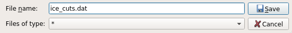
Launch the MCCS python script with your local python copy that includes pandas and shapely, and provide the file name that contains the ice cuts:
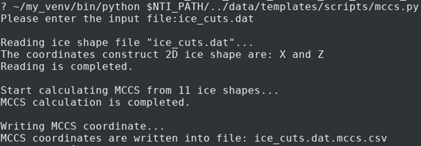
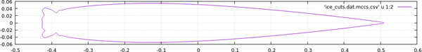
A new file will be created adding the suffix .mccs.csv to the original file name. This is a two-column text file where the values are separated by commas (CVS format).
You can plot the curve with your preferred data plotting software:
The files to open with Viewmerical can be specified on the command line.
Typical usages:
nti_3dview GRID3D gridfilenameLoads one grid.
nti_3dview GRID3D grid1 EOL GRID3D
                                grid2
Loads two grids, EOL is required to separate two commands.
nti_3dview SOLN3D gridfilename
                                solutionfile
Loads one grid & solution dataset.
nti_3dview SOLN3D gridfilename
                                    solutionfile:TEMP
Loads one grid & solution dataset, and loads the TEMP datafield (4-letter field identifier of FENSAP-style solution files).
nti_3dview ICE3DLoads map.grid, swimsol and ice.grid from the current directory.
Additional command syntax are listed in the -h all command-line help
output, however any command not listed in this user manual may not yet be fully
supported.