


The Ansys Chemkin Direct-Injection (DI) Diesel Engine Simulator is a variation of the spray-combustion model [60] that utilizes the detailed gas-phase chemistry to predict ignition timing and pollutant formations.
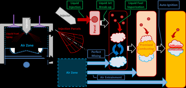
The spray-combustion model is a collection of phenomenological models that address the sequence of physical processes from liquid injection to vaporization in a direct-injection engine. The Chemkin DI Engine model largely follows the spray-combustion model HIDECS (Hiroshima University diesel engine combustion simulation) [60], [61] developed at the University of Hiroshima with small modifications to some of the sub-models. Figure 8.16: Physical and chemical processes included in the Chemkin DI Engine model provides a visual presentation of the physical and chemical processes included in the Chemkin DI Engine model. Short descriptions of individual sub-models implemented in the Chemkin DI Engine model will be given in the following sections. Detailed information about the spray-combustion model and the sub-models can be found in the papers by Hiroyasu et al. [60] , [61] and in the papers of similar spray-combustion DI engine models by Jung and Assanis [62] and by Bazari [63].
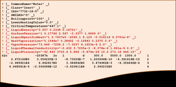
Thermodynamic and transport properties of the liquid species are fitted by various temperature functions. The exact functional form for each liquid property can be found in Fuel Library in the Ansys Forte User's Guide [64]. The liquid properties corresponding to a vapor/gas species are specified by special tags that must be placed before the gas-phase thermodynamic data of the vapor/gas species. The parameters given in the tags are coefficients of the temperature function for the specific liquid property. Any liquid fuel species involved in a DI engine simulation must have all the required liquid properties; the required liquid properties are density, specific heat capacity, the critical temperature, heat of vaporization, vapor pressure, surface tension, viscosity, and thermal conductivity. Properties of commonly-used liquid fuel species are already provided in the fuel library data file, fuel_library.inp, which must be included in the chemistry set of any DI engine simulation. The liquid species available in the fuel library are listed in Fuel Library in the Ansys Forte User's Guide . Properties of new liquid species can also be added to this fuel library data file. Figure 8.17: Prepending liquid properties to the corresponding vapor/gas species shows an example of how liquid properties are prepended to the corresponding vapor/gas species.
Injecting liquid into the hot air creates a highly non-uniform flow field in the engine cylinder. Since the conditions at the outer edges of the spray are very different from those at the center of the spray, it is desirable to have better spatial resolution of the spray to improve the solution accuracy. The spray-combustion model uses a Lagrangian scheme to describe the liquid spray and the surrounding hot air mixture. After the injection, the liquid spray is divided into concentric cones in the radial direction with respect to the centerline of the injector nozzle and into chunks in the injection direction. These parcels undergo various processes to transform from liquid to vapor individually as they travel at their own speeds inside the hot air mixture. Chemical reactions between the fuel vapor and the air and the occurrence of ignition in the parcel are determined by the detailed gas-phase reaction mechanism. Currently the air zone is treated as a single zone; it is possible to divide the air zone further to account for the temperature variation due to the wall heat loss. The air zone interacts with individual spray parcels explicitly through mass transfer due to the air entrainment process. Heat transfers amongst the spray parcels and the air zone are introduced by enforcing uniform cylinder pressure and the conservation of cylinder volume. There is no direct interaction between the spray parcels.
The spray parcels are adiabatic, and the wall heat loss is applied to the air zone only.
The Ansys Chemkin DI engine model solves the droplet variables (parcel penetration distance, droplet core temperature, and liquid component masses) and the gas-phase variables (gas temperature, gas mass, pressure, volume, and gas species mass fractions) of all spray parcels as a coupled ODE system; that is, no operator split scheme or sub-cycling/sub-time-stepping is employed. In order to run the simulations efficiently, it is important to keep the total number of spray parcels from exceeding a few hundred.
The sub-models employed by the Chemkin DI Engine model are briefly described next.
There are several phenomenological models employed by the Ansys Chemkin DI Engine model to describe some critical physics of the liquid fuel injection process. Because they are phenomenological models, they do not work perfectly under all the conditions, so calibrating model parameters is generally necessary.
The nozzle flow model is used to determine the conditions of the liquid jet at the outlet of the injector nozzles. The Chemkin DI Engine model uses the same nozzle flow model employed by Forte to determine the pressure drop across the nozzle and the liquid jet velocity at the nozzle outlet. Details of the nozzle flow model can be found in Spray Models in the Ansys Forte Theory Manual [65]. The liquid mass injection rate is fixed in the current version, alternative methods to describe variable injection mass flow rate will be implemented.
The Chemkin DI Engine model uses the correlation by Hiroyasu et al. [66] to estimate the liquid jet break-up time. A function is introduced to facilitate variations of the break-up time in the radial direction so that the liquid jet in the parcels at the edge of the spray will break earlier than those around the center of the spray.
 | (8–107) |
Where the radial distribution function is
 | (8–108) |
and Nr is the total number of parcels in the radial direction and m is the radial index of the parcel.
The correlation developed by Hiroyasu, Arai, and Tabada [67] is used to estimate the Sauter Mean Diameter (SMD) d32 of the droplets immediately after the break-up of the liquid jet. The initial SMD of the droplets is used to calculate the droplet population of the spray parcel.
 | (8–109) |
 | (8–110) |
 | (8–111) |
The penetration distance of the leading edge of the spray sp is determined by the empirical equations below [66]:
 | (8–112) |
 | (8–113) |
The radial distribution function ym is defined by Equation 8–108 . For simplicity, the model parameters in Equation 8–112 and Equation 8–113 are combined with the discharge coefficient of the injector nozzle Cd as suggested by Jung and Assanis [62].
The average speed of the liquid jet/droplets of a parcel is the time derivative of the penetration distance:
 | (8–114) |
 | (8–115) |
The mass flow rate from the air zone to the spray parcels can be derived by assuming that the momentum of the spray is conserved. The momentum at the start of liquid injections is equal to the total liquid fuel mass injected times the liquid jet speed at the nozzle exit:
 | (8–116) |
And the momentum of the spray parcel at a given time is the total mass of the spray times the parcel speed and is assumed to be the same as the initial momentum of the liquid jet:
 | (8–117) |
The total fuel mass in the spray remains constant because the fuel species simply transform from liquid to vapor and react to form new compounds. That is,
 | (8–118) |
By combining Equation 8–116 and Equation 8–117 , an expression for the air entrainment rate is obtained
 | (8–119) |
The spray parcels in the spray-combustion Direct Injection (DI) engine model can collide with each other and result in the redistribution of mass, composition, and energy. The interaction between the spray parcels, especially when there are multiple injections, can impact the ignition timings, the heat release rate characteristics, and the overall combustion efficiency.
The Ansys Chemkin DI Engine model employs a phenomenological parcel mixing model to obtain the average effects of the spray parcel interactions. Rather than trying to pair specific parcels and determine the mass exchange rate between them, the parcel mixing model allows the parcels to interact with each other indirectly through the air zone. The parcels interact with the air zone only. Firstly, a parcel releases its mass to the air zone at the mass flow rate determined by the parcel mixing model; the compositions and the enthalpies from all parcels will mix instantaneously because the air zone is well-stirred. This first step, the parcel back-mixing, simulates the overall mixing effect from the interactions among the spray parcels and the air zone. To complete the parcel interaction process, the contents of the air zone, representing the average result due to parcel interactions, will be distributed to the parcels by means of the air entrainment process described in the previous section.
The back-mixing mass flow rate from the individual parcel to the air zone in the first step of the parcel interaction process can be approximated by two factors: a driving force represented by a scalar gradient, between the parcel and the air zone, and a mixing frequency related to the velocity gradient. That is, the back-mixing mass flow rate from the j-th parcel to the air zone can be written as
 | (8–120) |
 represents the characteristic scalar mixing frequency,
  is the traveling speed of the j-th parcel and
 , the back-mixing coefficient, is a non-negative model parameter.
 is used as a measure of the scalar gradient between the
j-th parcel and the air zone. The parcel back-mixing can take place only
after the break-up of the liquid jet in the parcel, i.e.,
is used as a measure of the scalar gradient between the
j-th parcel and the air zone. The parcel back-mixing can take place only
after the break-up of the liquid jet in the parcel, i.e.,  . The back-mixing mass flow rate is expected to jump higher after the parcel
is ignited.
. The back-mixing mass flow rate is expected to jump higher after the parcel
is ignited.
Given the droplet surface temperature, the film theory of the evaporating droplet suggests that the vaporization rate of a liquid component is essentially the mass transfer rate of the vapor species across the boundary layer between the droplet and surrounding gas:
 | (8–121) |
Where the Spalding mass transfer number BM,k and the diffusional film correction factor FM,k(BM,k) are defined as
 | (8–122) |
 | (8–123) |
 and
and  are the gas density and the mass diffusivity of the vapor species
corresponding to the k-th liquid component in the thin-film
layer surrounding the droplet, respectively. The Sherwood number is computed as
are the gas density and the mass diffusivity of the vapor species
corresponding to the k-th liquid component in the thin-film
layer surrounding the droplet, respectively. The Sherwood number is computed as
 | (8–124) |
 | (8–125) |
 | (8–126) |
Where f(Re)=1 at Re⩽1 and f(Re)=Re0.077 at Re<100.
Since the vaporization rate calculation requires the droplet surface temperature, the Ansys Chemkin DI engine model employs two methods to estimate the droplet surface temperature. The first method assumes the droplet surface temperature is the same as the droplet core temperature, and the droplet core temperature will be solved by the energy conservation of the droplet. The second method allows the droplet surface temperature to be different from the droplet core temperature. While the droplet core temperature is still solved from the energy conservation equation, the droplet surface temperature will be solved iteratively by calculating the energy balance at the droplet surface.
At the droplet surface, the heat flux coming from the hot gas mixture surrounding the droplet is split into two parts. A portion of the energy is consumed by the vaporization process as the latent heat, and any surplus energy will be passed into the droplet to raise the droplet core temperature.
 | (8–127) |
The heat flux from the gas to the droplet surface can be obtained from
 | (8–128) |
The Spalding heat transfer number BT is correlated to the Spalding mass transfer number BM by [68]
 | (8–129) |
Where the parameter ϕ is given as
 | (8–130) |
and LE∞ is the Lewis number of the surrounding gas mixture.
The modified Nusselt number is computed from
 | (8–131) |
 | (8–132) |
 | (8–133) |
Since evaluating the correlation parameter ϕ requires BT , Equation 8–129 is solved iteratively until a converged BT value is obtained.
The heat flux penetrating into the liquid droplet can be estimated by the correlation given by Abramzon and Sirignano [68]
 | (8–134) |
Where  and
and  .
.
PeL = Re L Pr L is the Peclet number of the liquid droplet.
Currently, the droplet surface temperature is the same as the droplet center temperature
and  is set to zero.
The droplet temperature and the liquid species masses of an average droplet in each spray parcel are solved by the conservation laws.
The mass conservation equation is applied to each liquid fuel component. The liquid mass flow
rate at the nozzle outlet  and the vaporization rate
  are the two factors that affect the mass of a liquid species:
 | (8–135) |
 is the mass fraction of the liquid species
i
of the original liquid fuel mixture.
is the mass fraction of the liquid species
i
of the original liquid fuel mixture.
The temperature at the center of the droplet Td is solved by the energy conservation equation
 | (8–136) |
Ts is the droplet surface temperature.
The number of droplets after the break-up of the liquid jet is assumed to be constant during the vaporization process so that the instantaneous droplet diameter can be computed from the remaining liquid mass and the fixed droplet number. The droplet number is determined by the initial liquid mass and the Sauter Mean Diameter (SMD) of the initial droplet created when the liquid jet breaks up:
 | (8–137) |
And the droplet diameter after the break-up is computed by
 | (8–138) |