


Rate-dependent plasticity describes the flow rule of materials, which depends on time. The deformation of materials is now assumed to develop as a function of the strain rate (or time). An important class of applications of this theory is high temperature creep. Several options are provided in Mechanical APDL to characterize the different types of rate-dependent material behaviors. The creep option is used for describing material creep over a relative long period or at low strain. The rate-dependent plasticity option adopts a unified creep approach to describe material behavior that is strain rate dependent. Anand's viscoplasticity option is another rate-dependent plasticity model for simulations such as metal forming. Other than other these built-in options, a rate-dependent plasticity model may be incorporated as user material option through the user-programmable feature.
For information about the creep options available, see Rate-Dependent Plasticity (Viscoplasticity) in the Material Reference.
Also see Extended Drucker-Prager (EDP) Creep Model and Cap Creep Model.
The rate-dependent plasticity model includes four options: Perzyna([296]), Peirce et al.([297]), EVH([245]), and Anand([160]). The options are defined via the TB,RATE command’s TBOPT field (where TBOPT = PERZYNA, PEIRCE,
EVH, and ANAND, respectively), and are available with most current-technology
elements.
The material hardening behavior is assumed to be isotropic. The integration of the material constitutive equations are based a return mapping procedure (Simo and Hughes([252])) to enforce both stress and material tangential stiffness matrix are consistent at the end of time step. A typical application of this material model is the simulation of material deformation at high strain rate, such as impact.
The following topics describe each rate-dependent plasticity option:
The Perzyna option has the following form:
 | (4–95) |
where:
 = equivalent plastic strain rate = equivalent plastic strain rate |
| m = strain rate hardening parameter (input as C1 via TBDATA command) |
| γ = material viscosity parameter (input as C2 via TBDATA command) |
| σ = equivalent stress |
| σo = static yield stress of material (defined via TB,BISO, or TB,NLISO commands) |
Note: σo is a function of some hardening parameters in general.
As γ tends to
 , or m tends to zero
or
, or m tends to zero
or
 tends to zero, the solution converges to the static (rate-independent)
solution. However, for this material option when m is very small (<
0.1), the solution shows difficulties in convergence (Peric and Owen([298])).
tends to zero, the solution converges to the static (rate-independent)
solution. However, for this material option when m is very small (<
0.1), the solution shows difficulties in convergence (Peric and Owen([298])).
The Peirce option has the following form:
 | (4–96) |
Similar to the Perzyna model, the solution converges to the
static (rate-independent) solution,
as γ tends to
 , or m tends to zero, or
 tends to zero. For small value of m, this option
shows much better convergency than PERZYNA option (Peric
and Owen([298])).
tends to zero. For small value of m, this option
shows much better convergency than PERZYNA option (Peric
and Owen([298])).
For information about this option, see Exponential Visco-Hardening (EVH) Option in the Material Reference.
Metal under elevated temperature, such as the hot-metal-working problems, the material physical behaviors become very sensitive to strain rate, temperature, history of strain rate and temperature, and strain hardening and softening. The systematical effect of all these complex factors can be taken into account and modeled via Anand viscoplasticity([160], [148]). The Anand option is categorized into the group of the unified plasticity models where the inelastic deformation refers to all irreversible deformation that can not be simply or specifically decomposed into the plastic deformation derived from the rate-independent plasticity theories and the part resulted from the creep effect. Compare to the traditional creep approach, the Anand option introduces a single scalar internal variable "s", called the deformation resistance, which is used to represent the isotropic resistance to inelastic flow of the material.
Although the Anand option was originally developed for the metal forming application ([160], [148]), it is however applicable for general applications involving strain and temperature effect, including but not limited to such as solder join analysis, high temperature creep etc.
The inelastic strain rate is described by the flow equation as follows:
 | (4–97) |
where:
 = inelastic strain rate tensor = inelastic strain rate tensor |
 = rate of accumulated equivalent plastic strain = rate of accumulated equivalent plastic strain |
S, the deviator of the Cauchy stress tensor, is:
 | (4–98) |
and q, equivalent stress, is:
 | (4–99) |
where:
| p = one-third of the trace of the Cauchy stress tensor |
| σ = Cauchy stress tensor |
| I = second order identity tensor |
| ":" = inner product of two second-order tensors |
The rate of accumulated equivalent plastic strain,
 , is defined as follows:
 | (4–100) |
The equivalent plastic strain rate is associated with equivalent stress, q, and deformation resistance, s, by:
 | (4–101) |
| A = constant with the same unit as the strain rate |
| Q = activation energy with unit of energy/volume |
| R = universal gas constant with unit of energy/volume/temperature |
| θ = absolute temperature |
| ξ = dimensionless scalar constant |
| s = internal state variable |
| m = dimensionless constant |
Equation 4–101 implies that the inelastic strain occurs at any level of stress (more precisely, deviation stress). This theory is different from other plastic theories with yielding functions where the plastic strain develops only at a certain stress level above yielding stress.
The evolution of the deformation resistance is dependent of the rate of the equivalent plastic strain and the current deformation resistance. It is:
 | (4–102) |
where:
| a = dimensionless constant |
| h0 = constant with stress unit |
| s* = deformation resistance saturation with stress unit |
The sign,
 , is determined by:
 | (4–103) |
The deformation resistance saturation s* is controlled by the equivalent plastic strain rate as follows:
 | (4–104) |
where:
 = constant with stress unit = constant with stress unit |
| n = dimensionless constant |
Because of the
 , Equation 4–102 is able to account for both strain hardening
and strain softening. The strain softening refers to the reduction
on the deformation resistance. The strain softening process occurs
when the strain rate decreases or the temperature increases. Such
changes cause a great reduction on the saturation s* so that the current
value of the deformation resistance s may exceed the saturation.
, Equation 4–102 is able to account for both strain hardening
and strain softening. The strain softening refers to the reduction
on the deformation resistance. The strain softening process occurs
when the strain rate decreases or the temperature increases. Such
changes cause a great reduction on the saturation s* so that the current
value of the deformation resistance s may exceed the saturation.
The material constants and their units specified for the Anand option are listed in Table 4.3: Material Parameter Units for the Anand Option. All constants must be positive, except constant "a", which must be 1.0 or greater. The inelastic strain rate in Anand's definition of material is temperature and stress dependent as well as dependent on the rate of loading. Determination of the material parameters is performed by curve-fitting a series of the stress-strain data at various temperatures and strain rates as in Anand([160]) or Brown et al.([148]).
Table 4.3: Material Parameter Units for the Anand Option
| TBDATA Constant | Parameter | Meaning | Units |
|---|---|---|---|
| 1 | so | Initial value of deformation resistance | stress, e.g. psi, MPa |
| 2 | Q/R | Q = activation energy | energy / volume, e.g. kJ / mole |
| R = universal gas constant | energy / (volume temperature), e.g. kJ / (mole - K | ||
| 3 | A | pre-exponential factor | 1 / time e.g. 1 / second |
| 4 | ξ | multiplier of stress | dimensionless |
| 5 | m | strain rate sensitivity of stress | dimensionless |
| 6 | ho | hardening/softening constant | stress e.g. psi, MPa |
| 7 |

| coefficient for deformation resistance saturation value | stress e.g. psi, MPa |
| 8 | n | strain rate sensitivity of saturation (deformation resistance) value | dimensionless |
| 9 | a | strain rate sensitivity of hardening or softening | dimensionless |
where:
| kJ = kilojoules |
| K = kelvin |
If h0 is set to zero, the deformation resistance goes away and the Anand option reduces to the traditional creep model.
Long term loadings such as gravity and other dead loadings greatly contribute inelastic responses of geomaterials. In such cases the inelastic deformation is resulted not only from material yielding but also from material creep. The part of plastic deformation is rate-independent and the creep part is time or rate-dependent.
In the cases of loading at a low level (not large enough to cause the material to yield), the inelastic deformation may still occur because of the creep effect. To account for the creep effect, the material model extended Drucker-Prager (EDP model) combines rate-independent EDP with implicit creep functions. The combination has been done in such a way that yield functions and flow rules defined for rate-independent plasticity are fully exploited for creep deformation, advantageous for complex models as the required data input is minimal.
We first assume that the material point yields so that both plastic deformation and creep deformation occur. Figure 4.16: Material Point in Yielding Condition Elastically Predicted illustrates such a stress state. We next decompose the inelastic strain rate as follows:
 | (4–105) |
where:

|

|

|
The plastic strain rate is further defined as follows:
 | (4–106) |
where:
 = plastic multiplier = plastic multiplier |
| Q = flow function that has been previously defined in Equation 4–64, Equation 4–65, and Equation 4–66 in Extended Drucker-Prager Model |
Here we also apply these plastic flow functions to the creep strain rate as follows:
 | (4–107) |
where:
 = creep multiplier = creep multiplier |

As material yields, the real stress should always be on the yielding surface, implying that:
 | (4–108) |
where:
| F = yielding function defined in Equation 4–64, Equation 4–65, and Equation 4–66 in Extended Drucker-Prager Model |
| σ Y = yielding stress |
It is assumed that material hardening is
related to plasticity only and not to creep. The yield
stress,  , evolves as a function of the hardening
variable,
, evolves as a function of the hardening
variable,  :
:

where the hardening variable is the plastic work and is calculated from the summation of:

The creep behaviors could be measured through a few simple tests such as the uniaxial compression, uniaxial tension, and shear tests. We here assume that the creep is measured through the uniaxial compression test described in Figure 4.17: Uniaxial Compression Test.

The measurements in the test are the vertical stress
 and vertical creep strain
 at temperature T. The creep test
is targeted to be able to describe material creep behaviors in a general
implicit rate format as follows:
at temperature T. The creep test
is targeted to be able to describe material creep behaviors in a general
implicit rate format as follows:
 | (4–109) |
We define the equivalent creep strain and the equivalent creep stress through the equal creep work as follows:
 | (4–110) |
where:
 and and
 = equivalent creep strain and equivalent creep stress to be defined. = equivalent creep strain and equivalent creep stress to be defined. |
For this particular uniaxial compression test, the stress and creep strain are:
 | (4–111) |
Inserting (Equation 4–111) into (Equation 4–110) , we conclude that for this special test case the equivalent creep strain and the equivalent creep stress just recover the corresponding test measurements. Therefore, we are able to simply replace the two test measurements in (Equation 4–109) with two variables of the equivalent creep strain and the equivalent creep stress as follows:
 | (4–112) |
Once the equivalent creep stress for any arbitrary stress state is obtained, we can insert it into (Equation 4–112) to compute the material creep rate at this stress state. We next focus on the derivation of the equivalent creep stress for any arbitrary stress state.
We first introduce the creep isosurface concept. Figure 4.18: Creep Isosurface shows any two material points A and B
at yielding but they are on the same yielding surface. We say that
the creep behaviors of point A and point B can be measured by the
same equivalent creep stress if any and the yielding surface is called
the creep isosurface. We now set point B to a specific point, the
intersection between the yielding curve and the straight line indicating
the uniaxial compression test. From previous creep measurement discussion,
we know that point B has
 for the
coordinate p and
for the
coordinate p and
 for the coordinate q. Point B is now also on the
yielding surface, which immediately implies:
for the coordinate q. Point B is now also on the
yielding surface, which immediately implies:
 | (4–113) |
It is interpreted from (Equation 4–113) that
the yielding stress σ
Y is the function of the equivalent creep stress
 . Therefore, we have:
 | (4–114) |
We now insert (Equation 4–114) into the yielding condition (Equation 4–108) again:
 | (4–115) |
We then solve (Equation 4–115) for the equivalent
creep stress
 for material point A on the isosurface but with any arbitrary coordinates
(p,q). (Equation 4–115) is, in general, a nonlinear
equation and the iteration procedure must be followed for searching
its root. In the local material iterations, for a material stress
point not on the yielding surface but out of the yielding surface
like the one shown in Figure 4.16: Material Point in Yielding Condition Elastically Predicted, (Equation 4–115) is also valid and the equivalent creep
stress solved is always positive.
for material point A on the isosurface but with any arbitrary coordinates
(p,q). (Equation 4–115) is, in general, a nonlinear
equation and the iteration procedure must be followed for searching
its root. In the local material iterations, for a material stress
point not on the yielding surface but out of the yielding surface
like the one shown in Figure 4.16: Material Point in Yielding Condition Elastically Predicted, (Equation 4–115) is also valid and the equivalent creep
stress solved is always positive.

When the loading is at a low level or the unloading occurs, the material doesn’t yield and is at an elastic state from the point view of plasticity. However, the inelastic deformation may still exist fully due to material creep. In this situation, the equivalent creep stress obtained from (Equation 4–115) may be negative in some area. If this is the case, (Equation 4–115) is not valid any more. To solve this difficulty, the stress-projection method shown in Figure 4.19: Stress Projection is used, where the real stress σ is multiplied by an unknown scalar β so that the projected stress σ* = βσ is on the yielding surface. The parameter β can be obtained by solving the following equation:
 | (4–116) |
Again, Equation 4–116 is a nonlinear equation
except in the linear Drucker-Prager model. Because the projected stress σ* is on the yielding surface, the equivalent creep
stress denoted as
 and calculated by inserting σ* into (Equation 4–115), as follows:
 | (4–117) |
is always positive. The real equivalent creep stress
 is obtained by simply rescaling
 as follows:
 | (4–118) |
For creep flow in this situation, (Equation 4–107) can be simply modified as follows:
 | (4–119) |
For stress in a particular continuous domain indicated by the shaded area in Figure 4.19: Stress Projection, the stresses are not able to be projected on the yielding surface (that is, Equation 4–116) has no positive value of solution for β). For stresses in this area, no creep is assumed. This assumption makes some sense partially because this area is pressure-dominated and the EDP models are shear-dominated.
Having Equation 4–105,Equation 4–106, Equation 4–107, or Equation 4–119, Equation 4–108, Equation 4–110, and Equation 4–112, the EDP creep model is a mathematically well-posed problem.

The cap creep model is an extension of the cap (rate-independent plasticity) model. The extension is based on creep theory similar to that of the Extended Drucker-Prager (EDP) creep model.
Several concepts related to material creep theory (such as the equivalent creep stress, equivalent creep strain, and isosurfaces) are used in the cap creep model and are described in the EDP creep theory.
Unlike EDP which requires only one creep test measurement, a cap creep model requires two independent creep test measurements (as described in Commands Used for Cap Creep ) to account for both shear-dominated creep and compaction-dominated creep behaviors.
The following topics describing the cap creep model are available:
For related information, see Extended Drucker-Prager Cap Model and Extended Drucker-Prager (EDP) Creep Model in this reference.
The following assumptions and restrictions apply to the cap creep model:
Creep in both the shear and creep-expansion zones is measured via uniaxial testing.
The compaction creep zone is measured via hydrostatic testing.
Shear creep and compaction creep are independent of each other.
Shear creep exists in all zones insofar as possible.
The Lode angle effect is ignored.
Material hardening is dependent on plastic strain only.
The following yielding equation applies of the cap portion of the cap creep model:
 | (4–120) |
This equation represents the flow function of the cap creep model:
 | (4–121) |
The equations are similar to those used for yielding and flow function (respectively) in the cap (rate-independent plasticity) model.
The tension cap portion for the cap creep model is nearly identical to the cap (rate-independent plasticity) yielding function except that the J3 (Lode angle) effect is ignored. The notations and conventions remain the same.
Equation 4–120 is also used to calculate the equivalent creep stresses, and Equation 4–121 is used to calculate the creep strain.
For the sake of convenience, the cap domain shown in the following figure is divided into six zones (labeled 1, 2, 3, 10, 20, and 30):
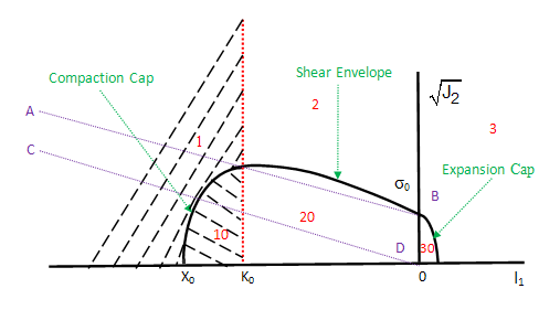
Following is a brief description of each zone:
Zone 1 shows the compaction zone where the material yields and creeps. Zone 10 represents a compaction-dominated zone; its inelastic behavior is still subject to a certain degree of creep due to compaction stress.
Zone 2 shows the shear zone where the material yields and creeps due to the shear effect. Zone 20 represents an elastic shear creep zone.
Zone 3 shows the expansion zone with both yield and creep. Zone 30 represents an elastic creep zone.
Creep in zones 2, 20, 3, and 30 is measured via uniaxial compression testing. Those zones do not experience compaction creep contributed from the compaction cap.
Zones 1 and 10 may also experience shear creep because a certain amount of shear creep exists in all zones. It is assumed that stress points below line CD are not subject to shear creep.
The shear and expansion zones share the same uniaxial compression for creep measurement. The derivation for the equivalent creep stress for the two zones is similar to that used for extended Drucker-Prager creep stress.
In coordinate system
 shown in the following figure, the coordinates
of the stress points from the uniaxial compression test are
shown in the following figure, the coordinates
of the stress points from the uniaxial compression test are
 , where
 is the measured stress or the equivalent creep stress.
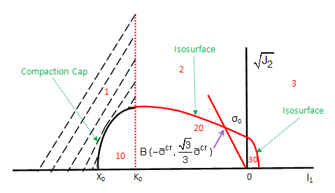
The point also on the shear yielding surface should satisfy the corresponding yielding function, as follows:
 | (4–122) |
or
 | (4–123) |
Equation 4–123 implies
 , which is used in the yielding condition

resulting in:
 | (4–124) |
Equation 4–124 is then solved for the equivalent
creep stress
 for stresses at either the shear zone or the expansion zone. As
shown in the EDP creep model, the measured creep strain component in the axial direction
is the equivalent creep strain; therefore, the creep rate function
for both shear and expansion zones is:
for stresses at either the shear zone or the expansion zone. As
shown in the EDP creep model, the measured creep strain component in the axial direction
is the equivalent creep strain; therefore, the creep rate function
for both shear and expansion zones is:

where
 is the equivalent creep strain
for the shear or expansion zone and
T is the temperature.
is the equivalent creep strain
for the shear or expansion zone and
T is the temperature.
The equivalent creep stress for compaction cap is assumed to be independent of J2 and only related to the first invariant of stress:

The creep test measurement for the compaction cap is regulated via hydrostatic compression testing. The measurement and record are
 where p is the hydrostatic
pressure, and
where p is the hydrostatic
pressure, and where
where
 is the volume
creep strain.
is the volume
creep strain.
Thus, the creep rate function for the compaction cap is:
 | (4–125) |
In zones 30, 20, 10, and 1 (where the material does not yield at the shear envelope criterion), loading is light; it also possible that unloading occurs. Inelastic deformation may still exist, however, due exclusively to material shear creep. In such a case, the equivalent creep stress obtained from the previous derivation may be negative. To avoid a negative equivalent creep stress, the stress-projection method proposed in EDP Elastic Creep and Stress Projection is used.
To model cap creep, use the input from the cap (rate-independent plasticity) model. The cap creep model ignores any tension-to-compression-strength ratio values and sets them to 1.
Creep data is input via the TB,CREEP command. Because the cap creep model requires two independent creep function inputs, an additional material table data command, TBEO, allows shear and compaction creep data to be defined separately.