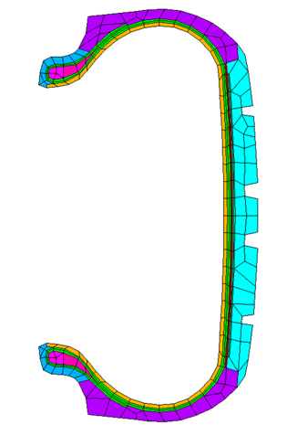
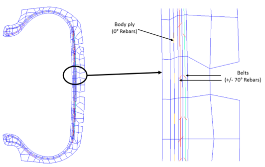
Reinforcings in the belt and body-ply regions are modeled with REINF263 smeared-reinforcing elements:

Figure 57.4: Tire Model Reinforcings

For the purpose of demonstration, both methods for defining reinforcing are used in this problem. The belt 1 reinforcings are created via the mesh-independent method, and the belt 2 reinforcings are created via the standard method.

! Create reinforcing elements at Belt_1
a1 = 0.22e-06       ! Cross-section area
s1=1.1e-03          ! Spacing
m1=10               ! Material number

sectype,9,reinf,smear		
secdata,m1,a1,s1,,-70,mesh	! Use "Mesh" pattern

et,2,200
keyopt,2,1,0
secn,9                           ! Use reinforcing section for Mesh200
mat,m1
type,2	

lsel,s,,,355,358                 ! Select lines representing reinforcing locations
cm,belt1_lines,line	
lmesh,all                        ! Mesh selected lines with MESH200 
allsel,below,line
cm,belt1_mesh200,elements
allsel,all

cmsel,s,belt1                    ! Select base elements in the belt1 region
cmsel,a,belt1_mesh200            ! Select MESH200 elements
mat,m1
ereinf                           ! Create reinforcing elements
allsel,all

! Delete Mesh200 elements after creating the reinforcing elements:
cmsel,s,belt1_lines	
lclear,all,all 
etdel,2 
allsel,all

! Creating reinforcing elements at Belt_2
a2 = 0.22e-06          ! Cross-section area
s2=1.1e-03             ! Spacing
m2=10                  ! Material number

sectype,11,reinf,smear			
secdata,m2,a2,s2,,70,edgo,1,.5
cmsel,s,belt2          ! Select base elements in the belt2 region
eplot
secnum,11
mat,10
ereinf                 ! Create reinforcing elements
allsel,all

The 2D axisymmetric tire model has two contact pairs:

The contact pair between the rim and the tire is initially made as a frictionless contact pair in the 2D axisymmetric model:

Figure 57.5: Rigid-Flexible Contact Pair Between Rim and Tire

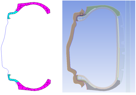
After the 2D axisymmetric analyses, the contact pair is converted to a bonded type contact pair for further analyses on the 3D model, as no relative motion is needed between the rim and the tire during steady-state rolling.

The rim is modeled as a rigid body. If required during the 2D to 3D analysis, other contact settings for this contact pair can be changed. In this example problem, convergence issues during rebalancing are resolved by adjusting the pinball radius.

The contact pair between the road and the tire plays no role in the 2D axisymmetric analyses:

Figure 57.6: Rigid-Flexible Contact Pair Between Road and Tire

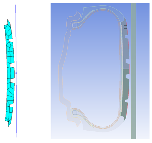
After the 2D axisymmetric analyses when the model is extruded to 3D, this contact pair is converted for the 3D model. Initially, the contact pair is frictionless. During the steady-state rolling load step on the 3D model, the coefficient of friction is gradually increased from 0 to 1.

The contact pair uses a default value representing the allowable elastic slip (SLTO). If problems occur when trying to obtain a free-rolling solution, you can override the default SLTO values by defining a scaling factor (a positive value when using command input) or an absolute value (a negative value when using command input).

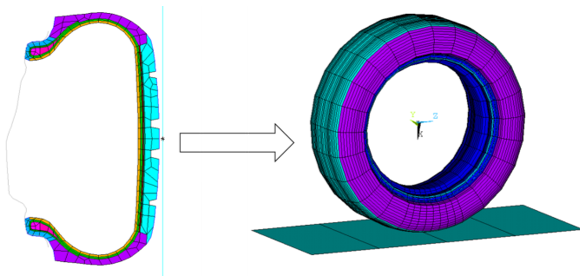
After the rim-mounting and inflation analyses on the 2D model, both contact pairs are extruded when the 2D model is converted to the 3D model. The rim surface is extruded in the circumferential direction, and the road surface is extruded in the global Z direction:

Figure 57.7: 2D Axisymmetric Tire Model Extruded to 3D

After performing the analyses on the 2D model, some contact settings for the contact pairs can be modified if necessary. For example: