


The suction-pile simulation involves three sequential analyses:
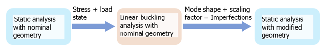
The following topics describe each of the analyses in the suction-pile simulation, including the boundary conditions, loading, and results for each:
A nonlinear static analysis with nominal geometry is performed. The analysis accounts for a specific loading history to obtain a loading and stress state suitable for use in the subsequent buckling analysis.
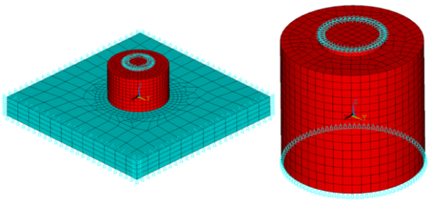
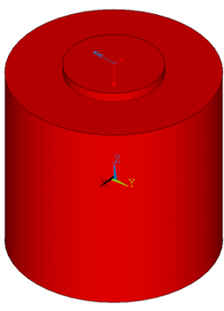
The bottom nodes of the soil and suction-pile skirt are fixed in a vertical direction.
Displacement in the perpendicular direction is restricted on all four sides of the underground model.
Displacement in the horizontal direction is restricted on top outer ring of the suction pile.
Loading occurs over four steps:
An initial in-situ earth pressure is generated by applying a gravitational acceleration of g = 9.81 m/s2 to the soil.
The in-situ stress-state calculation leads to undesirable vertical deformations. To mitigate the problem, an initial stress state is applied, resulting in a nearly deformation-free initial state for the gravitational load step.
Typically, soil exists in an already-consolidated state. Initial displacements due to at-rest loads are therefore unnatural and should be minimized. The vertical stress state SZ varies linearly based on the soil depth. SZ is determined via the soil density ρ, the gravitational acceleration g, and the vertical height h of each element:

The coefficient of lateral earth pressure is defined as the ratio of horizontal- to vertical-stress components. For a horizontally-retained non-overconsolidated soil under elastic loading conditions, the coefficient is defined via Poisson’s ratio ν:

The horizontal stress components are then determined by:

The known stress state is applied as the initial state (INISTATE).
Example 58.1: Applying an Initial Stress State
/solu ! Enter the solution processor

time, 1

! Specify the data type to be set on the subsequent INISTATE,DEFINE command
INISTATE,SET,DTYP,STRE

! Define stresses to the selected elements
INISTATE, DEFINE,,,,, Cxx, Cyy, Czz, Cxy, Cyz, Cxz

! Activate the file output of the calculated stress state at solution
inistate, write, 1, , , , , S

…

! Solve the first load step
solve

finish
Following is the resulting vertical-pressure distribution:
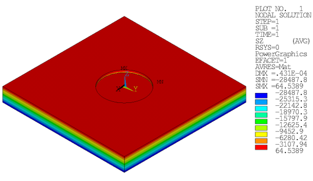
The initial at-rest pressure state is correctly applied, while the soil structure retains its initial shape.
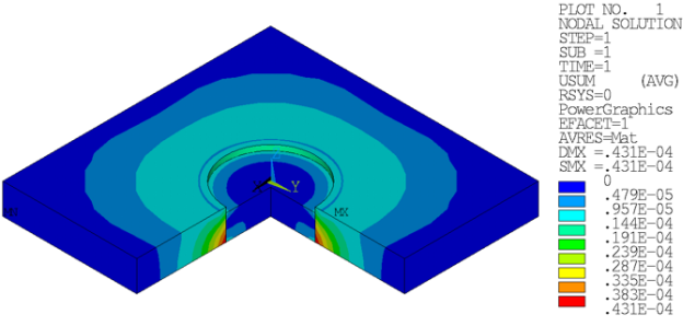
Marginal displacements (<0.5 mm Figure 6) are acceptable due to unbalanced soil pressure inside and/or outside of the soil region and contact penetrations:
A gravitational acceleration of 9.81 m/s2 is applied to the suction pile.
Forces caused by interaction with the upper structure are applied to the suction-pile top. Forces/moments are distributed over the top of the pile via contact pairs (CONTA174 / TARGE170) with the pilot-node option enabled.
| Upper Structure Interaction Load | ||
|---|---|---|
| Force / Moment |
Value
(kN; kN.m-1) |
| Fx | -5500.0 | |
| Fy | 200.0 | |
| Fz | -13000.0 | |
| Mx | -300.0 | |
| My | -3500.0 | |
| Mz | -50.0 | |
Suction pressure is applied on both the suction-pile skirt and lid. Constant pressure on the suction-pile skirt is assumed.
| Suction Pressure | ||
|---|---|---|
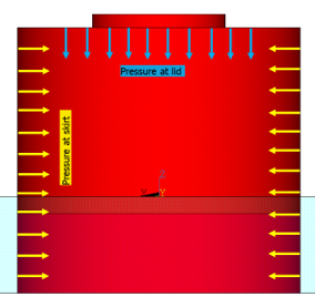
| Pressure Operation | Value (kPa) |
| At lid | 210.0 | |
| At skirt | 150.0 | |
Assumed frictional forces are applied on the suction-pile skirt where the skirt interacts with the soil.
| Frictional Forces | ||
|---|---|---|
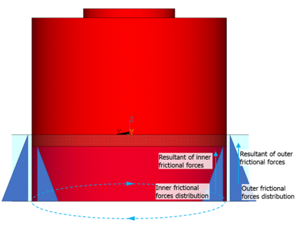
| Vertical Force Resultant | Value (kN) |
| At outer surface | 500.0 | |
| At inner surface | 500.0 | |
A nonlinear static analysis is performed. The in-situ stress state (load step 1) is calculated in a single substep.
Load steps 2 through 4 are calculated with automatic time-stepping enabled.
Initial-stress-state results are documented in Loading. Following are the results after load step 4:
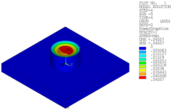
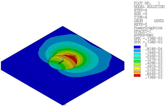
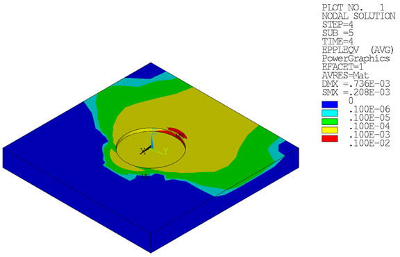
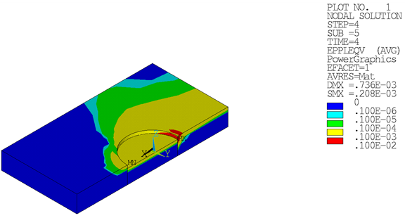
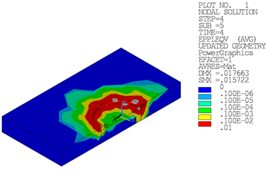
Loading on the suction pile leads to plastic strains in the soil. Plastic strains are distributed unsymmetrically due to unsymmetrical loading in load step 3 and load step 4:
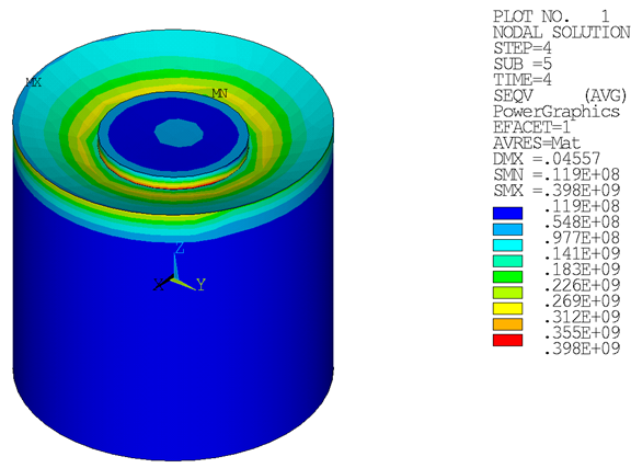
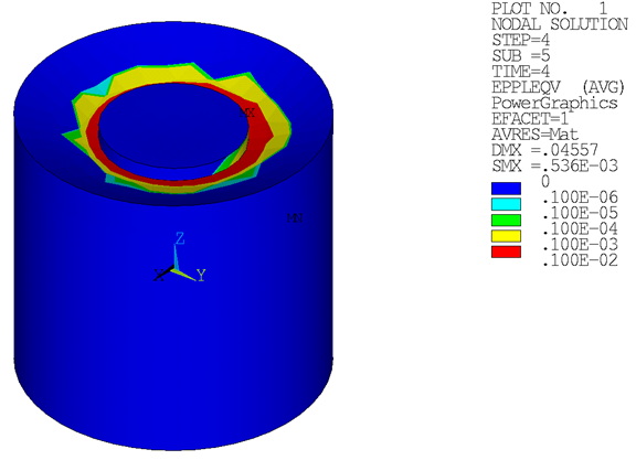
Strain on the suction pile causes plastic strains at the neck of the suction-pile cap:
Following the nonlinear static analysis with nominal geometry, a linear buckling analysis with nominal geometry is performed to obtain potential stability modes related to the static loads. The results are used as the basis for defining imperfections.
Boundary conditions from the prior static analysis are used.
A final load state from load step 4 in the prior static analysis is used as a reference load.
The linear buckling analysis is performed. Ten eigenmodes are calculated and expanded.
Example 58.2: Linear Buckling Analysis
finish

/clear

/assign,rstp,buckle,rst   ! Force Eigen analysis to write to buckle.rst

/solu

antype,static,restart,last,last,perturbation
perturb,buckle,,CURRENT,ALLKEEP  ! Nonlinear buckling analysis using
                                 !   loads from prestress analysis

solve, elform             ! Generate matrices needed for perturbation analysis

bucopt,subsp,10,,,center
outres,erase
outres,all,all
mxpand,10

solve
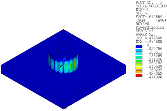
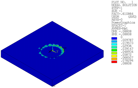
Ten eigenmodes were calculated during the buckling analysis. The resulting load factors range from 0.61086 to 1.1468.
The first buckling mode with a scaling factor of 0.135 is used to generate the structure imperfections:
A second nonlinear static analysis is performed using the updated geometry from the buckling analysis. To observe the influence of the added structural imperfections, the analysis uses the same loading from the first static analysis.
Boundary conditions from the first static analysis are used.
Loading is identical to that of the first static analysis. At the beginning of the analysis, however, the geometry is updated (UPGEOM) to account for imperfections (defined based on the buckling analysis results).
Example 58.3: Geometry Update (Adding Imperfections from the Buckling Analysis)
! Imperfections Resulting from Linear Buckling Analysis

esel,s,ename,,154
esel,a,ename,,170,174
esel,a,ename,,281
nsle
esln

UPGEOM,0.135,1,1,buckle,rst,
A nonlinear static analysis is performed, similar to the first, but using the updated geometry.
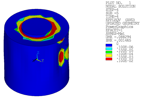
Following are the results after load step 4.
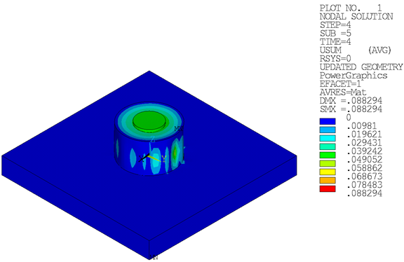
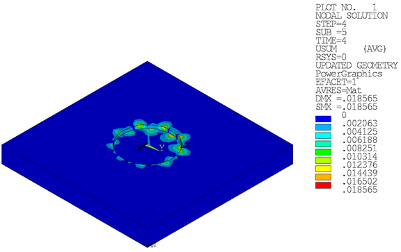
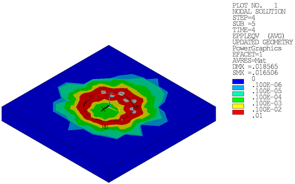
Compared to the static analysis results using nominal geometry, the analysis using the updated geometry with imperfections shows larger displacements and deformations on the suction-pile skirt, resulting in higher plastic strains:
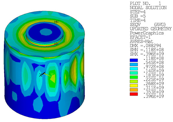
The suction-pile geometry without imperfections resulted in maximum plastic strains at the neck on the suction-pile cap. After including the imperfections, the same loading results in the critical region having moved from the suction-pile neck to the skirt:
Accounting for potential structural imperfections leads to qualitatively and quantitatively different results.