


The solution control and analysis settings are different for the full and CMS models. CMS generates substructures with generalized modal coordinates. This section describes substructure and CMS techniques for modal and harmonic analyses with the relevant analysis settings and solution controls.
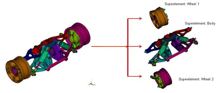
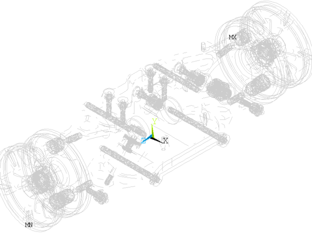
Substructuring is a procedure that condenses a group of finite elements into one element represented as a matrix. The single-matrix element is called a superelement. The substructure analysis uses the technique of matrix reduction to reduce the system matrices to a smaller set of degrees of freedom (DOFs). The use pass of a substructure reduces the computer time and enables the solution of very large problems with limited computer resources. The following figure shows how the suspension assembly is divided into three superelements: Wheel1, Wheel2, and Body.
A substructure analysis involves three distinct steps called passes: the generation pass, the use pass, and the expansion pass.
Generation pass
The objective of the generation pass is to condense a group of standard finite elements into a single superelement. The elements are condensed by identifying a set of master degrees of freedom (MDOFs) known as master nodes. Master nodes are used to define the interface between the superelement and the other elements and to capture the characteristics for the dynamic analyses.
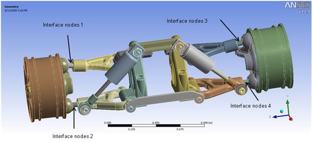
Proper choice of the interface master nodes is important to maintain continuity among the superelements and the other parts of the model. To optimize solution time, select the interface with the fewest nodes that still maintains continuity. For a 3D model, select the interface at a region of minimum cross-sectional area. For a 2D model, you would select the interface at a region of minimum length.
As shown in the following figure, the interface master nodes are defined on the shafts connecting the wheels and the body because the cross-sectional areas of the shafts are minimal compared to the other parts.
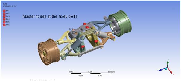
The Master nodes are also defined where boundary conditions or constraint equations are applied, as shown in the following figure:
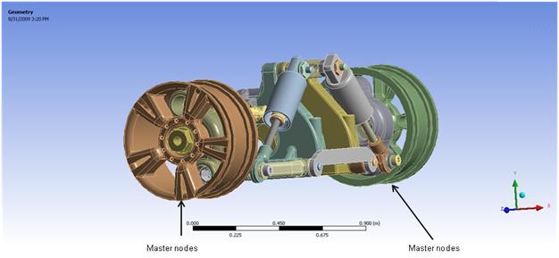
For the harmonic analysis, the points of load application are also defined as master nodes, as shown in this figure:
In the use pass (described below), the master nodes are the only nodes available for a superelement. The interface master nodes associated with Wheel1 and Body are named component “master1.” Master nodes associated with Wheel2 and Body are named component “master2”. In the substructure analysis, the superelement Wheel1 consists of the first wheel and the attached shafts up to “master1” and is termed Wheel1_for_solve. Likewise, the superelement Wheel2 consists of the second wheel and the attached shafts up to “master2” and is termed Wheel2_for_solve.
The following example input shows how the superelement of the first wheel is created after defining the master nodes:
/FILNAME, FIRSTWHEEL			! Name of the Superelement is FirstWheel
/SOLU
CMSEL, S, MASTER1, NODE		! Select a new set of interface nodal components named master1
M, ALL, ALL						! Define them as master nodes

/COM, SELECT A SET OF NODES FOR POINT OF APPLICATION OF HARMONIC DISPLACEMENT ON THE FIRST WHEEL
NSEL, S, NODE, , N1 			! Select the node n1 as a new subset
NSEL, A, NODE, , N2			! Additionally select the node n2 and extend the current set
NSEL, A, NODE, , N3			! Additionally select the node n3 and extend the current set
M, ALL, ALL						! Define them as master nodes

ALLSEL, ALL
CMSEL, ALL

NUM_MODES = 100					! Number of modes to extract for each component = 100
/SOLU
ANTYPE, SUBSTR					! Perform a substructure analysis
SEOPT, FIRSTWHEEL, 2			! Generate the stiffness and mass matrices
CMSOPT, FIX, NUM_MODES, 0, 100000	! Use fixed-interface method  to extract 100 modes between 0 and a
											! large number
CMSEL, S, WHEEL1_FOR_SOLVE		! Select a new subset of components to create the superelement
											! associated with the first wheel and the attached shaft
ESLN, S								! Select a new set of elements attached to the selected nodes
SOLVE
FINISH
SAVE
Use pass
The superelement is used to make it a part of the whole model. The entire model may be a superelement, or the superelement may be connected to non-superelements.
The solution from the use pass consists of only the reduced solution for the superelement, which is the DOF solution only at the MDOF, and the complete solution for non-superelements.
Expansion pass
The results at all DOFs in the superelement are calculated at the start of the expansion pass. If multiple superelements are used in the use pass, a separate expansion pass will be required for each superelement.
The reduced solution obtained from the use pass is applied to the model as displacement boundary conditions, and the complete solution within the superelement is solved.
The expansion pass logic for substructuring analysis searches for the superelement .LN22 file and, if found, uses the sparse solver to perform a back-substitution.
You can specify a load step and a substep for expanding a particular frequency (EXPSOL).
Using component mode synthesis (CMS), the dynamic characteristics of the full system model are formed by first formulating the dynamic behavior of each of the components, and then enforcing equilibrium and compatibility along component interfaces.
The generated substructure information in CMS is in the .sub file, which is all that is required in the use pass. Because the internal details of the structure are not exposed using CMS, specialized teams can work on the same structure without having to provide detailed or proprietary information about the component. The superelements created in the generation pass are combined in the use pass with knowledge of master nodes. The superelements are given a new element type: MATRIX50.
The following sample input shows how the superelements are combined in the use pass.
/FILNAME, USE
/PREP7
*GET, MAX_ETYPE, ETYP, , NUM, MAX		! Retrieve the value of the maximum element type number
															! and store it as MAX_ETYPE
ET, MAX_ETYPE+1, 50							! Define Matrix50 as the next element type number
TYPE, MAX_ETYPE+1								! Assign this type number to the elements
MAT, 1													! Assign 1 as the material number to subsequently defined
															! elements
REAL, MAX_ETYPE+1								! Set the element real constant set attribute pointer
SE, FIRSTWHEEL									! Define the superelement associated with the Wheel1
SE, BODY												! Define the superelement associated with the Body
SE, SECONDWHEEL									! Define the superelement associated with the Wheel2
FINISH
The following figure shows the resulting superelements:
A CMS substructure can be advantageous over a basic substructure because it is more accurate than a Guyan reduction for model, harmonic, and transient analyses. CMS includes truncated sets of normal modal generalized coordinates that characterize the behavior of the components of the structural model.
A typical use of CMS involves modal analysis of a large, complicated structure (such as an aircraft or nuclear reactor) where various teams are in charge of the design of a component of the structure. With CMS, design changes to a single component affect only that component; therefore, additional generation passes are necessary only for the modified substructure.
The following CMS options are available:
Fixed-interface (CMSOPT,FIX), where interface nodes are constrained during the CMS superelement generation pass.
Free-interface (CMSOPT,FREE), where interface nodes remain free during the CMS superelement generation pass.
Residual-flexible free-interface (CMSOPT,RFFB), where interface nodes remain free during the CMS superelement generation pass.
The fixed-interface CMS method is preferable for most analyses. The free-interface method and the residual-flexible free-interface method are useful when an analysis requires more accurate eigenvalue computation at the mid to high end of the spectrum. As in substructuring, a component mode synthesis analysis involves three distinct steps or passes. In CMS generation pass, a group of finite elements are condensed into a single CMS superelement that includes a set of master degrees of freedom (MDOFs) and truncated sets of normal mode generalized coordinates. The MDOFs serve to define the interface between the superelements and the other elements. The CMS use pass and expansion pass utilize the same procedure as a basic substructure analysis.
As multiple superelements were used for the present model in the use pass, a separate expansion pass would usually be required for each of them. However, since the response nodes belong to the superelement Body, expansion of this superelement is sufficient.
A modal analysis determines the natural frequencies and mode shapes of a structure. These are important parameters in the design for dynamic loading conditions, and required to perform a spectrum, mode-superposition harmonic, or transient analysis. Several mode-extraction methods are available: Block Lanczos, Supernode, PCG Lanczos, unsymmetric, damped, and QR damped. The damped and QR damped methods allow inclusion of damping in a structure. The QR damped method also allows for the unsymmetrical damping and stiffness matrices.
Modal analysis is a linear analysis aimed at finding the eigensolution; therefore, no force is involved in the modal analysis. Nonlinearities, such as plasticity and contact (gap) elements, are ignored even if they are defined. In this model, the Block Lanczos method is used to extract the modes with the boundary conditions shown in Figure 22.6: Master Nodes Defined at Fixed Bolts.
A harmonic analysis determines the steady-state response of a linear structure to loads that vary sinusoidally (harmonically) with time. The structure's response is determined over a range of frequencies and a response quantity (usually displacements) is plotted versus frequency. Peak responses are then identified on the graph, and stresses are reviewed at those peak frequencies.
This analysis technique calculates only the steady-state, forced vibrations of a structure. The transient vibrations, which occur at the beginning of the excitation, are not accounted for in a harmonic analysis. Harmonic analysis is typically linear. Some nonlinearities, such as plasticity are ignored, even if they are defined; however, unsymmetric system matrices (such as those encountered in a fluid-structure interaction problem ) can be accommodated in the harmonic analysis.
In the present model, base excitation is applied in the form of sinusoidal displacement in the vertical y-direction at selected nodes on both wheels. Those nodes are defined as master nodes in the generation pass (as shown in Figure 22.3: Suspension Assembly with Boundary Conditions and Displacement Loading and Figure 22.7: Master Nodes Defined at Points of Application of Harmonic Displacement).
The response is calculated at the response nodes specified during the expansion pass, as shown in this figure:
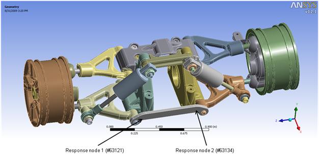
As the response nodes belong to only one of the superelements (Body), the results file of Body is used for the response calculation. The following example input performs the expansion pass with postprocessing:
/CLEAR, NOSTART
/FILNAME, BODY			! Change the jobname to Body
RESUME, ,					! Resume the database file Body.db
/SOLU
EXPASS, ON					! An expansion pass will be performed
OUTRES, ALL, ALL			! Write the solution of the specified solution results item for
									! every substep in the database
SEEXP, BODY, USE			! Specify the name of the dsub file as use, containing the
	 								! superelement degree-of-freedom (DOF) solution
NUMEXP, ALL, , , 		! Expand all substeps with element results
SOLVE
SAVE
FINISH

/post26

/COM, NODES FOR RESPONSE CALCULATION
N7 = NODE(0.22701, -0.98593E-01, -0.35058)		! Select the node #63121 defined by the coordinates
N8 = NODE(0.22701, -0.98292E-01, 0.42245E-01) 	! Select the node #63134 defined by the coordinates

/VIEW, 1, 1, 1, 1				! Define the viewing direction as isometric
/SHOW, PNG							! Creates PNG (Portable Network Graphics) files that are
											! named Body001.png onwards
ALLSEL, ALL
NSOL, 7, N7, U, Y 				! Store the nodal data for N13 for y-displacement into the
											! variable 7
NSOL, 8, N8, U, Y 				! Store the nodal data for N14 for y-displacement into the
											! variable 8
PLVAR, 7								! Plot the data for variable 7
PLCPLX, 0							! Plot the amplitude of the complex variable
PLVAR, 8								! Plot the data for variable 8
PLCPLX, 0
PLVAR, 7, 8							! Plot the data for variables 7 and 8 in the same plot
PLCPLX, 0

/SHOW, CLOSE
FINISH