Both the modal and harmonic analyses are performed using full and CMS models, and their solution times are noted. Significant improvement in the solution time is observed for the CMS model with very little loss of accuracy.
Before the harmonic analysis, a modal analysis with the same boundary conditions is performed using both the full and CMS models. The following table compares the first 50 eigenfrequencies obtained using both methods:
Table 22.1: Comparison of Eigenfrequencies for Full and CMS Models
| Mode # | Full Model | CMS Fixed Interface | % Diff | Mode # | Full Model | CMS Fixed Interface | % Diff |
|---|---|---|---|---|---|---|---|
|
1 |
31.12 |
31.31 |
0.59 |
26 |
421.43 |
421.11 |
0.08 |
|
2 |
33.13 |
33.12 |
0.03 |
27 |
438.35 |
437.67 |
0.16 |
|
3 |
44.66 |
44.69 |
0.08 |
28 |
441.79 |
441.03 |
0.17 |
|
4 |
53.17 |
53.10 |
0.12 |
29 |
452.46 |
452.13 |
0.07 |
|
5 |
87.88 |
88.18 |
0.34 |
30 |
496.92 |
496.10 |
0.17 |
|
6 |
88.63 |
88.97 |
0.38 |
31 |
513.90 |
513.11 |
0.15 |
|
7 |
144.61 |
144.55 |
0.04 |
32 |
539.43 |
538.38 |
0.19 |
|
8 |
146.77 |
146.41 |
0.24 |
33 |
553.06 |
552.27 |
0.14 |
|
9 |
187.22 |
187.23 |
0.01 |
34 |
557.25 |
557.39 |
0.03 |
|
10 |
223.63 |
223.70 |
0.03 |
35 |
570.47 |
571.11 |
0.11 |
|
11 |
237.48 |
237.41 |
0.03 |
36 |
620.15 |
619.67 |
0.08 |
|
12 |
251.83 |
251.69 |
0.06 |
37 |
633.79 |
634.34 |
0.09 |
|
13 |
256.42 |
256.48 |
0.02 |
38 |
647.02 |
647.11 |
0.01 |
|
14 |
263.33 |
263.05 |
0.10 |
39 |
675.83 |
675.73 |
0.01 |
|
15 |
272.06 |
271.91 |
0.06 |
40 |
707.77 |
708.04 |
0.04 |
|
16 |
274.79 |
274.68 |
0.04 |
41 |
708.81 |
709.53 |
0.10 |
|
17 |
357.55 |
358.10 |
0.15 |
42 |
714.94 |
715.58 |
0.09 |
|
18 |
368.37 |
368.17 |
0.06 |
43 |
716.93 |
716.76 |
0.02 |
|
19 |
368.47 |
368.26 |
0.06 |
44 |
726.62 |
726.06 |
0.08 |
|
20 |
368.50 |
368.30 |
0.06 |
45 |
734.91 |
734.39 |
0.07 |
|
21 |
368.77 |
368.56 |
0.06 |
46 |
734.93 |
734.41 |
0.07 |
|
22 |
372.73 |
372.32 |
0.11 |
47 |
734.97 |
734.43 |
0.07 |
|
23 |
387.18 |
386.90 |
0.07 |
48 |
734.99 |
734.44 |
0.07 |
|
24 |
391.96 |
391.67 |
0.08 |
49 |
751.62 |
751.70 |
0.01 |
|
25 |
415.22 |
414.77 |
0.11 |
50 |
768.84 |
768.93 |
0.01 |
The following table shows the elapsed and CPU times for modal analysis using the full and CMS models for 100 frequencies. Significant improvement in solution time is achieved during the use pass via the CMS method.
Table 22.2: Comparison of CPU and Elapsed Times for Modal Analysis
| Number of Modes = 100 | Full Model | CMS Fixed Interface | |
|---|---|---|---|
| CPU Time (s) | 2034.280 | Gen Pass | 2022.670 |
| Use Pass | 4.630 | ||
| Elapsed Time (s) | 1291.000 | Gen Pass | 1336.000 |
| Use Pass | 3.000 | ||
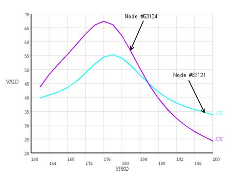
The harmonic analysis is conducted over the frequency range of 160 Hz to 200 Hz in 20 substeps. The following table compares the CMS and full model response amplitudes for the two response nodes.
Table 22.3: Comparison of Response Amplitudes for Full and CMS Models
| Node # 63121 | Node # 63134 | ||||||
|---|---|---|---|---|---|---|---|
| Freq (Hz) | Full Model | CMS Fixed Interface | % Diff | Freq (Hz) | Full Model | CMS Fixed Interface | % Diff |
| 162 | 39.65 | 39.7493 | 0.25 | 162 | 44.1064 | 43.7604 | 0.78 |
| 164 | 40.8758 | 40.896 | 0.05 | 164 | 48.6884 | 48.237 | 0.93 |
| 166 | 41.9754 | 41.9335 | 0.10 | 166 | 52.4358 | 51.9039 | 1.01 |
| 168 | 43.5616 | 43.4692 | 0.21 | 168 | 56.0015 | 55.4024 | 1.07 |
| 170 | 45.9102 | 45.7711 | 0.30 | 170 | 59.7247 | 59.0597 | 1.11 |
| 172 | 48.9518 | 48.7638 | 0.38 | 172 | 63.5063 | 62.7696 | 1.16 |
| 174 | 52.2104 | 51.9681 | 0.46 | 174 | 66.7185 | 65.905 | 1.22 |
| 176 | 54.7814 | 54.4813 | 0.55 | 176 | 68.2576 | 67.3727 | 1.30 |
| 178 | 55.668 | 55.3164 | 0.63 | 178 | 67.0837 | 66.1534 | 1.39 |
| 180 | 54.4876 | 54.1044 | 0.70 | 180 | 63.1036 | 62.1716 | 1.48 |
| 182 | 51.7678 | 51.3783 | 0.75 | 182 | 57.3466 | 56.4547 | 1.56 |
| 184 | 48.4247 | 48.0481 | 0.78 | 184 | 51.1398 | 50.3119 | 1.62 |
| 186 | 45.1665 | 44.8127 | 0.78 | 186 | 45.3776 | 44.6201 | 1.67 |
| 188 | 42.3427 | 42.0154 | 0.77 | 188 | 40.4304 | 39.7395 | 1.71 |
| 190 | 40.0521 | 39.7523 | 0.75 | 190 | 36.3475 | 35.7165 | 1.74 |
| 192 | 38.2657 | 37.9946 | 0.71 | 192 | 33.0387 | 32.4621 | 1.75 |
| 194 | 36.8948 | 36.6556 | 0.65 | 194 | 30.3676 | 29.8435 | 1.73 |
| 196 | 35.8121 | 35.6126 | 0.56 | 196 | 28.1851 | 27.7175 | 1.66 |
| 198 | 34.8474 | 34.7009 | 0.42 | 198 | 26.3318 | 25.9327 | 1.52 |
| 200 | 33.7753 | 33.7011 | 0.22 | 200 | 24.6321 | 24.3226 | 1.26 |
The following table shows the elapsed and CPU times for harmonic analysis using full and CMS models for 20 substeps. The use pass includes the expansion. Significant improvement in solution time is achieved via the CMS method.
Table 22.4: Comparison of CPU and Elapsed Times for Harmonic Analysis
| Number of Modes = 20 | Full Model | CMS Fixed Interface | |
|---|---|---|---|
| CPU Time (s) | 13580.800 | Gen Pass | 2022.670 |
| Use Pass | 1758.800 | ||
| Elapsed Time (s) | 7866.000 | Gen Pass | 1336.000 |
| Use Pass | 1764.000 | ||
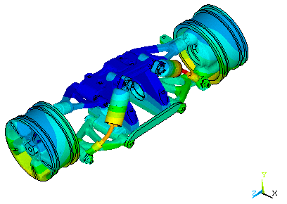
As shown in the following figure, the response amplitude plots for the two nodes show distinctive peaks at ~176 Hz.
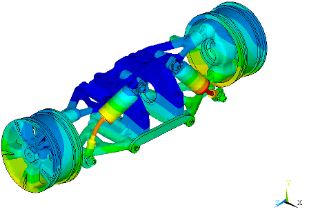
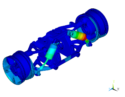
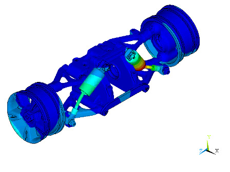
The peaks are explained by observing the mode shape at the undamped natural frequency of 187.22 Hz (Figure 22.11: Mode Shapes at the Undamped Natural Frequency of 187.22 Hz). The figure shows the configuration of the structure at two extreme deflections. The mode shape at this frequency has tilting vibrations of the wheels (in phase) about the x axis with the associated deflection of part of the body. Harmonic displacement at the bottom of the wheels in the Y-Direction excites this mode, resulting in peaks at nearby frequencies.
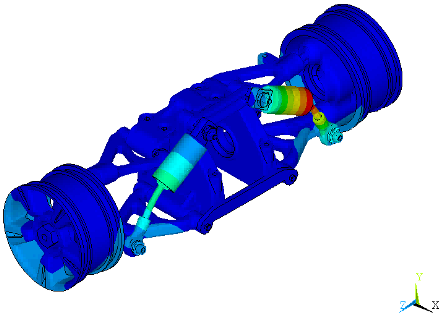
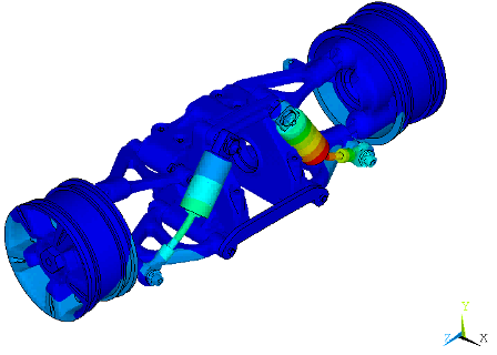
Mode shapes for nearby higher frequencies (223.63 Hz and 237.48 Hz) do not involve significant tilting of the wheels or deflection of the links attached to the response nodes. Figure 22.12: Mode Shapes at the Undamped Natural Frequency of 223.63 Hz and Figure 22.13: Mode Shapes at the Undamped Natural Frequency of 237.48 Hz show the mode shapes at these frequencies.