


In the process of additive manufacturing, parts are produced by sintering/fusing material in a track-by-track fashion compositing material horizontally into thin layers and then vertically into actual part geometry.
Additive Print's Mechanics Solver (the AP Mechanics Solver, or simply the Mechanics Solver) simulates this process of material consolidation into geometric shapes and the resulting distortions from intended shape and induced internal residual stresses. The manufacturing process involves depositing very thin tracks of material sequentially. But to simulate the micron level of detail relies upon a highly accurate thermal solution and huge amount of computing resources. To get a reasonably accurate solution in a faster manner the Mechanics Solver makes a set of simplifying assumptions.
Theory and Assumptions
The AP Mechanics Solver assumes that the entire powder layer is melted at once instead of in a track-by-track fashion. This melted layer sits on top of an existing solid layer and experiences thermal shrinkage during the solidification process. Cooling of the material is assumed to happen instantaneously. Multiple micron-scale physical layers are combined into one layer for simulating this shrinkage process. Each of these layers is meshed using the closest possible approximation of voxels, the size of which is defined by the input parameter, Voxel Size. This results in a voxelized representation of the actual geometry after all layers are meshed. Due to the thermal gradient across solidified layers and subsequent variable shrinkage, the material experiences internal stresses that get locked in as residual stresses.
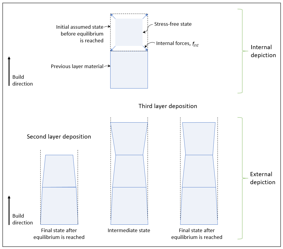
For a given deposition layer the shrinkage of the material can be written in equation form as:

where  is mechanical strain and
  is thermal strain.
Internal force in the material in this layer is generated as a resistance to thermal shrinkage:

where  is the strain displacement matrix and
  is elastic modulus.
 is obtained by assuming
  for the top layer to get
  . The actual value of
  and
and  are obtained after solving for global equilibrium. We can solve for equilibrium
across the geometry using:
are obtained after solving for global equilibrium. We can solve for equilibrium
across the geometry using:

where  is the global stiffness matrix and
  is the global displacement vector. This is a simple linear elastic formulation
to obtain a fast solution. For the plastic solution, to obtain equilibrium we use Newton-Raphson
iterations to reach a converged equilibrium solution. For that we calculate a yield function that
is dependent on current stress and plastic strain:
is the global displacement vector. This is a simple linear elastic formulation
to obtain a fast solution. For the plastic solution, to obtain equilibrium we use Newton-Raphson
iterations to reach a converged equilibrium solution. For that we calculate a yield function that
is dependent on current stress and plastic strain:

where  is the stress tensor,
  is the yield function,
  is the deviatoric stress tensor,
  is the equivalent plastic strain, and
  is the hardening modulus.
At every Newton-Raphson iteration the yield function is calculated to check for convergence:

A residual is calculated based on the internal force and used for convergence:

An incremental contribution to the total displacements is calculated based on this residual:

The final solution is based upon this cumulative of the incremental displacements. The total and elastic strains are calculated as:

The shrinkage strains are not applied to support material and omitting these strains reduces computation time. Overhang features are assumed to be either connected to the part or supported. If they are not, no strain will be applied to them until they are joined with the rest of the part. (See Hanging/Floating Voxels.) Nodes on the bottom of the part and support are fixed in place to represent the assumption that baseplate deflection is not significant with respect to part deflection.
Strain Modes
The structural problem of the additive simulation is driven by thermal shrinkage
( ) that results in part deformation and residual stresses. There are three strain
modes that the Mechanics Solver can use to drive it: assumed strain, scan pattern-based
anisotropic strain, and thermal strain. The assumed strain option applies isotropic inherent
strain to each layer for simulation. This inherent strain can be obtained from previously
calibrated parts. See the Additive Print and Science Calibration Guide. The scan pattern-based anisotropic strain
uses the scan paths for the laser and generates anisotropic directional dominant strains.
Experimental studies show that shrinkage strain is higher parallel to the scan direction than
perpendicular to the scan direction. The scan pattern strain mode can be used to apply this kind
of anisotropic strain based upon the scan vectors. The strains for the parallel,
perpendicular, and Z-directions are determined by multiplying the inherent strain by the
anisotropic strain coefficient. Directional strains for each scan are aggregated within each
individual voxel used in the structural solution to give location dependent strains. The strains
in the thermal strain option are generated by the Thermal Solver as explained in the following section.
) that results in part deformation and residual stresses. There are three strain
modes that the Mechanics Solver can use to drive it: assumed strain, scan pattern-based
anisotropic strain, and thermal strain. The assumed strain option applies isotropic inherent
strain to each layer for simulation. This inherent strain can be obtained from previously
calibrated parts. See the Additive Print and Science Calibration Guide. The scan pattern-based anisotropic strain
uses the scan paths for the laser and generates anisotropic directional dominant strains.
Experimental studies show that shrinkage strain is higher parallel to the scan direction than
perpendicular to the scan direction. The scan pattern strain mode can be used to apply this kind
of anisotropic strain based upon the scan vectors. The strains for the parallel,
perpendicular, and Z-directions are determined by multiplying the inherent strain by the
anisotropic strain coefficient. Directional strains for each scan are aggregated within each
individual voxel used in the structural solution to give location dependent strains. The strains
in the thermal strain option are generated by the Thermal Solver as explained in the following section.
Coupling with Thermal Solver
The Thermal Solver produces a rich spatio-temporal temperature field. This solver follows the laser path in small time intervals and simulates the thermal conduction through the solidifying part. The resulting temperature field is available at micron scale. The Mechanics Solver is weakly coupled with the Thermal Solver which means the temperature fields are used passively to simulate the mechanical response. Based on the time history of temperature at a given location, the Thermal Solver uses a thermal ratcheting method to modify the user-defined inherent strain and generate shrinkage strain values to pass to the Mechanics Solver. The Mechanics Solver reads the shrinkage strain data and averages it over the given mesh element and applies it as an unbalanced force boundary condition. The thermal ratcheting algorithm used to generate thermal strain is discussed in the following section.
Thermal Strain – Thermal Ratcheting Algorithm
This strain mode provides the highest degree of accuracy by predicting how thermal cycling affects strain accumulation at each location within a part. A "thermal ratcheting" algorithm assigns a base strain to each location within the part as it solidifies. Each time a location within the part is heated above a temperature threshold (approximately 40% of its absolute melting temperature) an increase in strain in that location occurs. If a location re-melts, the strain is reset to the base strain. The more times a location is heated above the threshold without melting, the higher the strain accumulates. Once the strain magnitude is calculated for each location within a part using the thermal ratcheting algorithm, that strain is passed to the Mechanics Solver and applied as an anisotropic strain based upon both local strain magnitude and local scan orientation. Because thermal strain requires a thermal prediction for every scan vector, this strain mode requires a much longer computational time. As in Assumed Strain and Scan Pattern simulations, you will need to calibrate for Strain Scaling Factor.
Post-processing of Simulation Results
After the additive manufacturing process, distortion and residual stress that result in a part create various problems and opportunities for improvement. Using simulation can inform your decision-making regarding how to set-up, prevent failures, and even compensate the geometry for best printing results. The Additive application's Mechanics Solver internally produces results that can be useful in various contexts. For example, warping results are used to find curling of the part in the vertical direction and a potential recoater blade crash is indicated in the blade crash result file. Relieving the part by cutting it off from the baseplate results in a release of some of the locked-in stresses and this rebalances the part's internal forces. This results in a re-distortion of the part. The Mechanics Solver can simulate this cutoff process and calculate the after cutoff distortion. The final distortion of the part can be used to invert the part to various magnitudes and rebuild to obtain a to-the-spec geometry. This kind of compensated geometry can be produced by the solver. Residual stresses at the part and support interface are used to generate an optimized support by changing the thickness of the support walls or change the distance between support walls. When the part is being built it undergoes a history of distortion and residual stresses. Some areas of the geometry may experience high stresses in one of the layers despite having a low final stress after deposition of all layers. This could be a result of rebalancing of stresses after further layers are deposited. This history of high stress might indicate internal/external cracking and some other microscopic defects. The Mechanics Solver can save the high-water mark of stresses and strains through the history and output for the entire geometry at the end of simulation. These high stresses and strains can be used to inspect and possibly change the geometry to mitigate failures.
Relationship Between the AP Mechanics Solver and the MAPDL Solver
The AP Mechanics Solver is the structural solver included in the Additive application. Everything written in this theoretical overview applies to the AP Mechanics Solver.
The Mechanical APDL (PCG) Solver is used for additive simulations in the Mechanical application. The FEA technology used by the AP Mechanics Solver is very similar to that of the Mechanical APDL (PCG) Solver, except for a few notable differences listed in the table below.
| Additive Print Mechanics Solver | Mechanical APDL Solver In Mechanical |
| The bottom of the build is automatically constrained. | The bottom of the build is typically connected to a baseplate. The user applies a fixed condition to the baseplate. |
| Inherent strain is applied to the part only starting from the second layer. | Inherent strain is applied to the part and supports starting from the first layer. |
| Strain is not applied to unconnected overhangs, such as “stalactite” points, lines, and surfaces (also known as islands), until the voxels are connected to voxels that touch the base. | Strain is applied to unconnected overhangs. |
| Nodal results displayed at the interface between support and part elements show results averaged from part elements only. | Nodal results displayed at the interface between support and part elements show results averaged from both part and support elements. |
Starting at Release 2020 R2, the Mechanical APDL Solver was implemented in the Additive application as the solver just for the specific case of displacement after cutoff, including both instantaneous and directional cutoff options.