


The Thermal Solver simulates scan tracks on each deposit layer of the Laser Powder Bed Fusion (LPBF) additive manufacturing process. The solver takes a multi-scale approach, leveraging periodic behavior observed in LPBF to improve performance. At the fine scale, a transient FEM solution is used to determine a temporally evolving temperature field. The fine-scale solution is then coarsened out to apply a periodic heating solution to each deposit layer of the entire build, while still following the laser path.
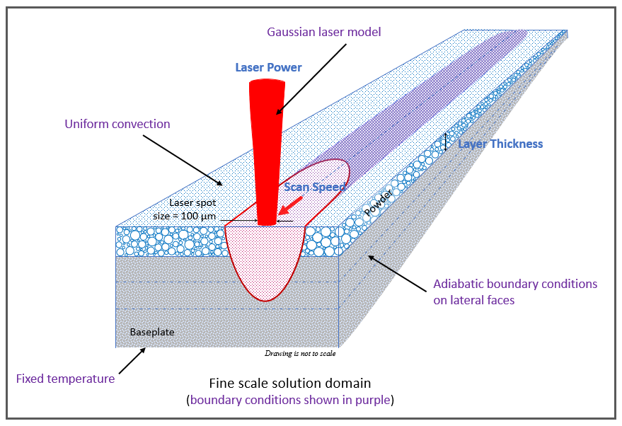
The fine-scale solution is an FEM simulation of diffusion in a single scan track. The material properties (such as conductivity, density, specific heat) are temperature-dependent and state-dependent for powder and the bulk solid. Powder properties are a ratio of the bulk-solid properties, and the ratio may also be temperature dependent. The powder is treated as a homogeneous absorbing scattering medium in which a Gaussian laser model is applied as a volumetric heat source along the top of this track (see Gusarov et. al. [1]). An absorption coefficient and extinction coefficient are used to model the energy penetration for a given scan speed and laser power combination, as found from the material tuning process.
The mesh in the FEM solution is not the same voxel mesh as used in the Mechanics Solver. Rather, it is a Cartesian grid with uniform horizontal resolution and a different grid resolution in the build direction determined dynamically based upon the deposit layer thickness. The horizontal mesh resolution is different for various simulation types. However, these fine-scale mesh resolutions are not user adjustable so if a melt pool becomes too large and reaches the domain boundaries, edge effects may appear.
Going from the fine-scale single-track result to the part level, the horizontal mesh resolution is coarsened by a Mesh Resolution Factor (MRF) to improve performance. The MRF is user adjustable for some simulation types. Too large of an MRF may result in poor resolution of melt pools. At the part level, each deposit layer starts out as all powder at the ambient heater temperature. The MRF-coarsened heating solution is applied to each individual solution step within each scan track in the scan pattern. Cooling is simulated during the scans as well as during the inter-scan dwell time between tracks. The mesh nodes marked as powder become melted once the temperature exceeds the material's solidus value. Once a node is melted, the material state is no longer powder and this history is retained through successive layers.
The user-specified Baseplate Temperature is used as a fixed-temperature boundary condition at the bottom of the build. In addition to the Gaussian laser heat-source model, the top boundary of the build has a constant forced convection applied uniformly. Aside from the laser model, radiation effects are neglected. The lateral boundary conditions are adiabatic while using a buffer region of powder extending out from the part's bounding box to avoid any boundary effects.
The current approach has its limitations. As periodic behavior is a key assumption for performance, only fill-type scans can be simulated well in terms of simulation runtime. The solver can predict lack-of-fusion porosity via the powder-solid state tracking but does not predict balling or keyhole phenomena. Other physical phenomena that are not explicitly modeled include: latent heat, surface tension effects, vaporization, plasma, and spatter. As such, an experimentally determined "cap temperature" is found for each alloy as part of the material tuning process. This cap temperature will offset some of the adverse effects of the assumptions and limitations.
Thermal Solver Default Settings
Simulations using the Thermal Solver have some input parameters that are not available to the user. These variables include thermal material properties, mesh size, absorptivity, and laser penetration depth. Thermal material properties are temperature dependent and have been set to match material produced through the additive manufacturing process. Laser penetration depth and absorptivity have been tuned to fit data from single bead experiments and vary according to the power and velocity used in the simulation. Mesh size is set to 15 µm for Single Bead, Thermal Strain, Microstructure and Thermal History simulations, and 25 um for Porosity simulations. These values have been identified as values that give good results both in terms of accuracy and simulation speed.
Re-tuning of the Ansys predefined materials may or may not be performed each software release, depending on the extent of the solver updates. When material re-tuning is performed, small changes in results from previous releases may be observed.
With Additive's user defined material capability, you can examine trends and create your own materials that account for these variations in absorptivity and penetration depth. Documentation is available that describes the theory and procedure, including the use of the Material Tuner tool (Beta) that automates much of the simulation work for you.
Guidelines for Resolving Warnings and Errors
As the model is not completely user adjustable, some errors may arise. This section discusses some potential issues you may encounter.
Edge effects in highly diffusive materials and/or high energy density scenarios
The fine-scale scan track domain width and depth have been set based on tuning of commonly used build settings and are not user adjustable. Process-parameter inputs that provide a very large energy density may result in edge effects due to the boundary conditions applied to the fine-scale single track solution. Melt pool width and depth growth may be impeded by the adiabatic lateral boundaries and constant temperature bottom boundary, respectively, under extreme conditions. That is, melt pool dimensions may become artificially constrained. This presents in different ways depending on the material's diffusivity.
For highly diffusive materials, such as Aluminum alloys, if the melt pool width or depth approaches the domain boundary exceeding a set tolerance, the solver logs a warning or errors-out with a message describing which dimension(s) triggered the failure.
For less diffusive materials, the melt pool growth may not be sufficient to trigger the warning/error but may still be constrained by domain edge effects. In this scenario, the solution continues. The way to discern the phenomena is to observe that the melt pool dimension(s) does not change as the energy into the system continues to increase.
If either scenario is encountered, we recommend reducing the input energy density (any combination of reducing the Laser Power, or increasing the Scan Speed or Laser Beam Diameter) or selecting a material with a lower diffusivity.
Specifically, this behavior has been observed when the melt pool width and/or the melt pool depth approach certain limits. For width, this is on the order of ∼600 microns, and becomes more severe as it approaches ∼800 microns. Due to differences in sensitivity to melt pool depths for different simulation types, the onset for this issue will vary from melt pool depths of ∼400 microns for Single Bead, Porosity, and Microstructure simulations; to ∼200 microns for Thermal History (Beta) and ∼140 microns for Thermal Strain simulations. We do not expect this issue of edge effects to be present under typical operating ranges for most simulation types, that is, using typical process parameters. It is typically only when you "push the boundaries" of the operating window that you may experience these edge effects. But we believe testing the boundaries is exactly what simulation is for, so we do not necessarily discourage it. To serve as a potential alert that you may be pushing the boundaries, we include recommended ranges that are tighter than allowable ranges for the process parameters that affect energy density most directly: Laser Power and Scan Speed. For example, the allowable range for Laser Power is 50 to 700 Watts but a range of 50 to 500 Watts is shown in the UI as the "recommended range." The following simulation types may be affected in the following ways:
Thermal Strain: The thermal strain may be less accurate, affecting the quality of the resulting stress and distortion. It should be noted that while Thermal Strain simulations use a shallower mesh and are more likely to be influenced by this on a localized basis, the overall impact is mitigated by the averaging that occurs when preparing to run a structural solution.
Single Bead: The reported melt pool width and depth may be artificially capped at around 800 microns and 400 microns, respectively.
Porosity: The resulting solid ratio may be under-predicted.
Microstructure: The resulting melt pool width and depth may be under-predicted, and the thermal gradients and cooling rates may be incorrect.
Thermal History (Beta): The reported melt pool width and depth may be under-predicted, and average temperature may be less accurate.
Warnings related to Mesh Resolution Factor
The Mesh Resolution Factor (MRF) is user adjustable for some simulation types. Too large of an MRF will lead to poor resolution of the melt pool. The Thermal Solver will emit a warning when this occurs. A smaller MRF may resolve the melt pool and should resolve the warning, at the cost of longer simulation times.