Plot settings are largely similar for all plot types. Each plot can be configured through the Plot Properties dialog. The Plot Properties dialog has two tabs, General and Legend. The General tab is where the results component and geometry scope are defined. It possible to configure a plot to display only a particular section of a component. The Legend tab controls the format of the plot legend. Specific to solution plots is the selection of the solution set of interest.

The General Tab has the following properties:

The Legend tab allows you to control titles, labels, and legend ranges:

Failure plots show the critical values for all defined failure criteria (modes) and integration points. The strain and stress plot illustrates the values at the element center (interpolation). Therefore, the absolute strain and stress peaks are not displayed in the plots and the elements have a constant value. This can cause graphical inconsistency between the strain/stress and failure plot.

Displays nodal deformation results and can plotted for the following:

Shows strain values at the bottom, mid, or top position of the ply and at the element center (or at the bottom or top of the laminate if ply-wise is disabled). In the Ansys Mechanical application, this corresponds to the Elemental Mean display option. Strains can be displayed ply-wise or for an entire laminate. Strain results can be plotted for the following component directions:

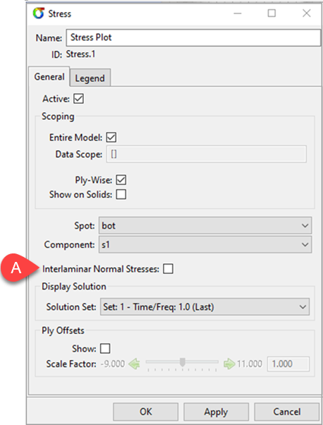
Displays stress values at the bottom, mid, or top position of the ply and at the element center (or at the bottom or top of the laminate if ply-wise is disabled). This corresponds to the Elemental Mean display option in the Ansys Mechanical application. There is an option to compute Interlaminar Normal Stresses for shell elements as explained in Interlaminar Stresses.

Interlaminar Normal Stresses: (see A, below) Activates a separate post-processing step to compute the interlaminar normal stresses s3 for shell elements. This happens automatically if a 3D failure criterion is active (for example: Puck 3D or Max Stress s3). Note that the s3 stresses are cached once they are evaluated because the computation can be costly. Use Delete Post-Processing Results from the solution’s action menu to clear the cache. By default, s3 stresses are available for solid elements. See Interlaminar Normal Stresses in the theory chapter for more information.

Stress results can be plotted for the following stress component directions:

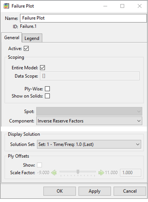
Failure plots can be used to display the safety factor for first ply failure of a pre-defined failure criteria definition. Failure results can be displayed in the following ways:

The failure evaluation for each defined failure criterion uses stress or strain results at each integration point. In contrast, stress and strain plots display the elemental mean results.

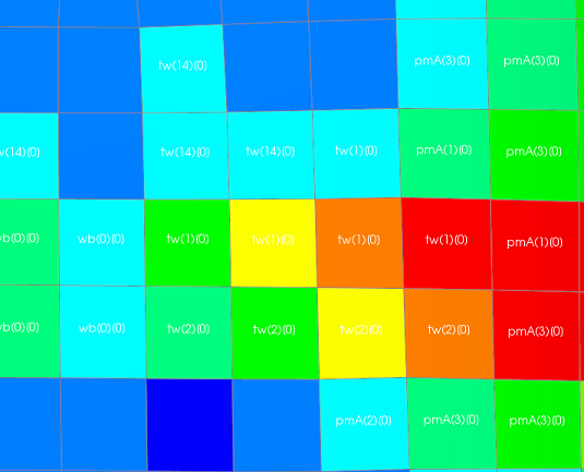
There are three kinds of safety factors that can be displayed in a failure contour plot. Text labels can be activated to show the critical failure mode and in what layer it occurs. In the case of an envelope solution, the critical load case can also be shown. The toolbar button   switches the display of activated element text labels on and off. For information on failure definitions see Postprocessing.

Available safety factor components:

The failure plot properties have the following additional options:

Figure 2.167: Scene with Failure Mode Plot Activated

The temperature plot can display a temperature field results on solid elements if temperature data is available in the results file.

This plot object can display progressive damage results. The overall damage status can indicate if, and how much, damage has occurred. The damage variables indicates how much the stiffness has reduced for fiber and matrix in tension or compression. The damage variable scale goes from 0 (no damage, 0% stiffness reduction) to the maximum stiffness reduction specified. The highest reduction possible is 1 (complete damage, 100% stiffness reduction).

Note that a failure analysis for this analysis type should be done with care and may not make sense for damaged elements.

See Damage Results in the Mechanical User's Guide for more information on each result component.

The following components can be plotted:

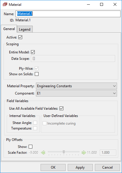
The Material Plot enables you to visualize ply-wise variable material properties.

Figure 2.168: Material Plot General Properties Tab

By default, all available field variables are used to evaluate the selected material property. However, you can also deactivate some of these variables to inspect the dependency of the selected material property more easily with respect to some specific factors. During the evaluation, inactive variables stay fixed at their default value.

Available field variables include the Shear Angle (defined by draping simulation in ACP-Pre), Temperature (if temperature data is available in the results file), and your own variables defined using Field Definitions in ACP-Pre.

For this plot type, the plot-specific options of the General tab include:

This plot object can be used to plot a scalar data set provided as a Python list or numpy.ndarray , as well as associated custom text labels, provided as a list of strings. Once the plot has been loaded, you can query active element indices, labels, and respective element centroid coordinates through the plot user interface properties based on the data scope. User-defined plots can be created as a lay-up plot or a solution plot. The plot is defined using the Python interface. The code can be placed in the script field of the plot object. This ensures the plot is refreshed following model updates. Alternatively, the plot definition can be executed through the Python shell. For more information about the Python interface, see The ACP Python Scripting User Interface.

Figure 2.169: Script Field in the User-Defined Plot Properties

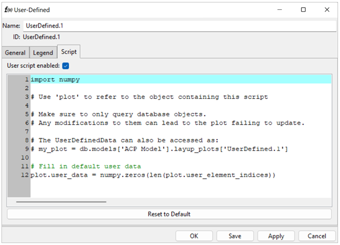
In addition to the default buttons (OK, Apply, and Cancel), the Script has a Save button which saves the modifications without closing the window or updating the model.

Python User Interface Properties

Example Scripts

A few examples of user-defined plots are shown in this section. The Python scripts are delivered with the installation of ACP. You will find them in this location:

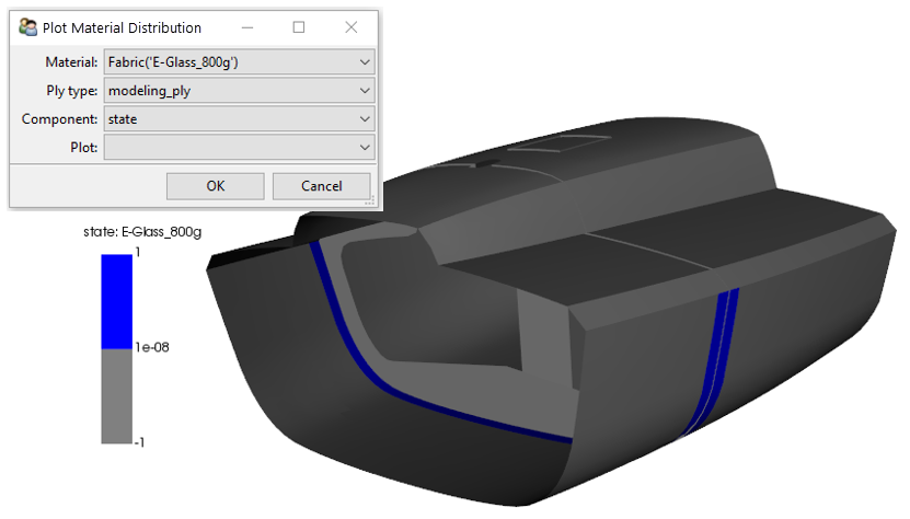
Example 2.1: Show Material Distribution

Script: C:\Program Files\ANSYS Inc\v242\ACP\script_examples\MaterialDistributionPlots\Wizard\material_plot_main.py

This plot shows the material distribution of a specific material in the structure. You can choose to plot the total thickness of all plies of this material, the number of plies, or just 0/1 per element as shown below. You make your selection using a simple wizard. To generate the plot, select File > Run Script… and then choose the script material_plot_main.py. The wizard creates the user-defined plot. Afterwards, you can use the Script tab to change parameters.

The next examples are based on the class40.wbpz Workbench workshop. Each example consists of two parts: the first part configures the user-defined plot, and the second part sets the user-script of the plot. These scripts are also included with your ACP installation: (C:\Program Files\ANSYS Inc\v242\ACP\script_examples).

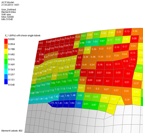
Example 2.2: Plot Material Property Distribution

Script: C:\Program Files\ANSYS Inc\v242\ACP\script_examples\plot_material_property_distribution.py

The sample code provided shows you how to create an advanced material plot which you can use to plot variable material data. In this case, the objective is to plot variable material data with a custom label, using the user-defined Plot to do so. The example below plots the effective Young's modulus as a function of draping simulation with shear angle labels.

• This project contains a material called E_Glass_shear_dependent.

• This material is contained within cell B5 (ACP) of class40.wbpz.

Open ACP Setup of cell B5 and either run the script (File > Run Script …) or follow the instructions below to create the user-defined plot.

1. The following commands must be copied and pasted (CTRL-Shift-V) into the Python shell in ACP.

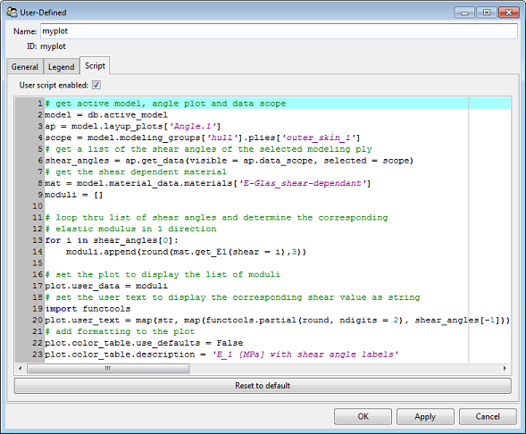
   # get active model
   model = db.active_model
   # get angle plot
   ap = model.layup_plots['Angle.1']
   # set the angle plot to display the draped shear angle
   ap.component =  'shear'
   # set the plot data scope to modeling ply 'outer_skin_1' which uses a draping simulation
   scope = model.modeling_groups['hull'].plies['outer_skin_1']
   ap.data_scope = scope
   # update the model
   model.update()
   
   # create a user defined lay-up plot
   up = model.layup_plots.create_user_defined_plot(name = 'myplot')
   # apply the same scope as before
   up.data_scope = scope
   # enable the script field
   up.user_script_enabled = True
   up.show_user_text = True
   
   

2. The following code must be placed within the Script field of UserDefinedPlot object myplot:

   # get active model, angle plot and data scope 
   model = db.active_model 
   ap = model.layup_plots['Angle.1'] 
   scope = model.modeling_groups['hull'].plies['outer_skin_1'] 
   plot.data_scope = [scope] 
   # get a list of the shear angles of the selected modeling ply 
   shear_angles = ap.get_data(visible = ap.data_scope, selected = scope) 
   # get the shear dependent material 
   mat = model.material_data.materials['E-Glas_shear-dependant'] 
   moduli = [] 
   
   # loop thru list of shear angles and determine the corresponding 
   # elastic modulus in 1 direction 
   for i in shear_angles[0]: 
       moduli.append(round(mat['engineering_constants'].query('E1', {'Shear Angle' : i}),3)) 
   
   # set the plot to display the list of moduli  
   plot.user_data = moduli 
   # set the user text to display the corresponding shear value as string, rounded to 2 digits 
   import functools 
   plot.user_text = list(map(str, map(functools.partial(round, ndigits = 2), shear_angles[-1]))) 
   # add formatting to the plot 
   plot.color_table.use_defaults = False 
   plot.color_table.description = 'E_1 [MPa] with shear angle labels'
   

This script should result in the following plot:

Example 2.3: Plot Combined Shear Stress Values- User-Defined Failure Criteria

Script: C:\Program Files\ANSYS Inc\v242\ACP\script_examples\plot_user_defined_combined_shear_stresses.py

The sample code below shows how you can plot the margin against the combined interlaminar shear stresses.

Open ACP Setup of cell B5 and either run the script (File > Run Script …) or follow the instructions below to create the user-defined plot.

1. The following commands must be copied and pasted (CTRL-Shift-V) into the Python shell in ACP.

   # get active model
   model = db.active_model
   # set data scope to element set
   scope = model.element_sets['HULL_BELWL']
   
   # create a stress plot for out-of-plane shear stress s13
   sp = model.solutions['Solution 1'].plots.create_stress_plot()
   sp.data_scope = scope
   sp.component = 's13'
   
   # create a second stress plot for out-of-plane shear stress s23
   sp1 = model.solutions['Solution 1'].plots.create_stress_plot()
   sp1.data_scope = scope
   sp1.component = 's23'
   # update the model, to make stress data available
   model.update()
   
   # create user defined solution plot
   up = model.solutions['Solution 1'].plots.create_user_defined_plot(name = 'myplot.1')
   # apply the same data scope as before
   up.data_scope = scope
   up.user_script_enabled = True
   

2. The following code must be placed within the script field of the UserDefinedPlot object myplot:

   # import numpy extentsion for mathematical operations
   import numpy
   # get active model, set data scope as before and select core layer
   model = db.active_model
   scope = model.element_sets['HULL_BELWL']
   ply = model.modeling_groups['hull'].plies['core_bwl'].production_plies['ProductionPly.9'].analysis_plies['P1L1__core_bwl']
   
   # retrieve references to stress plots created before
   sp = model.solutions['Solution 1'].plots['Stress.1']
   sp1 = model.solutions['Solution 1'].plots['Stress.2']
   
   # get list of s13 and s23 stresses
   s13 = sp.get_data(visible = sp.data_scope, selected = ply)[0]
   s23 = sp1.get_data(visible = sp1.data_scope, selected = ply)[0]
   
   # take the sqrt of the sum of squares
   combined = numpy.sqrt(numpy.power(s13,2) + numpy.power(s23,2))
   # define a stress limit
   slimit = 1.1
   
   # calculate the inverse reserve factors (irfs)
   irf = combined / slimit
   
   # set the plot to display the list of irfs
   plot.user_data = irf
   # add formatting to the plot
   plot.color_table.use_defaults = False
   plot.color_table.description = 'irf_plot'
   

This script should result in the following plot:

Example 2.4: Mesh Selections and Queries on a Solid Model

User-defined plots can also show results on solid elements. The sample code below shows how to execute mesh selections and mesh queries for solids.

1. The following commands must be deployed from within the UI of cell B5:

   # get active model
   model = db.active_model
   # set data scope to element set 'BULKHEAD_ALL'
   scope = model.element_sets['BULKHEAD_ALL']
   
   # create a user defined lay-up plot and apply the data scope set before
   up = model.layup_plots.create_user_defined_plot(name = 'myplot.2')
   up.data_scope = scope
   # enable the script field
   up.user_script_enabled = True
   # activate the solid model display option
   up.show_on_solids = True
   

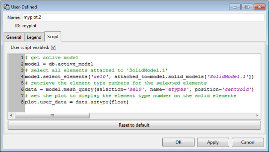
2. The following code must be placed within the script field of the UserDefinedPlot object myplot.2:

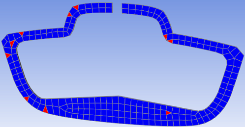
   # get active model
   model = db.active_model
   # select all elements attached to 'SolidModel.1'
   model.select_elements('sel0', attached_to=model.solid_models['SolidModel.1'])
   # retrieve the element type numbers for the selected elements using a mesh query
   data = model.mesh_query(selection='sel0', name='etypes', position='centroid')
   # set the plot to display the element type number on the solid elements
   plot.user_data = data.astype(float)
   

This script should result in the following plot. The prism and brick elements are highlighted separately:

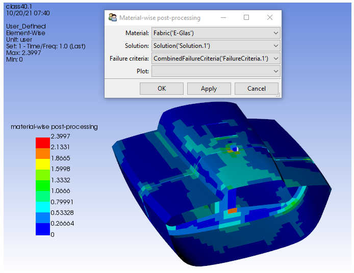
Example 2.5: Material-wise Post-Processing

This example shows how to generate a failure plot that computes the most critical failure within an element for a specific material or a list of materials. For instance, you could determine the most critical failure of all uni-directional materials per element.

Script: C:\Program Files\ANSYS Inc\v242\ACP\script_examples\ MaterialWisePostProcessing\material_wise_post_processing.py

To generate the plot, select File > Run Script… and then choose the script failure_plot_main.py. This opens a wizard which allows you to configure parameters such as material, solution, and failure definition. To further customize it, use the Script tab in the Property dialog of the user-defined plot. For instance, you might choose to select a list of materials instead of a single material.

Script: C:\Program Files\ANSYS Inc\v242\ACP\ script_examples\MaterialWisePostProcessing\material_wise_post_processing.py

This script generates a template of a user-defined plot for material-wise post-processing. Within the script of the user-defined plot, you can adjust the parameters such as the materials and the solution. In this example, you can also select a list of materials.