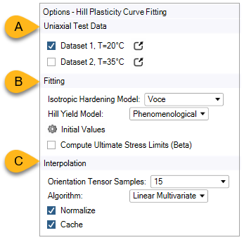
Uniaxial Test Data: (A in the figure above.) You can select one or multiple Datasets among those defined in the Experimental Data. If only one experimental Dataset is selected, setting the temperature value is optional. If multiple Datasets are selected, each must be at a different Temperature.

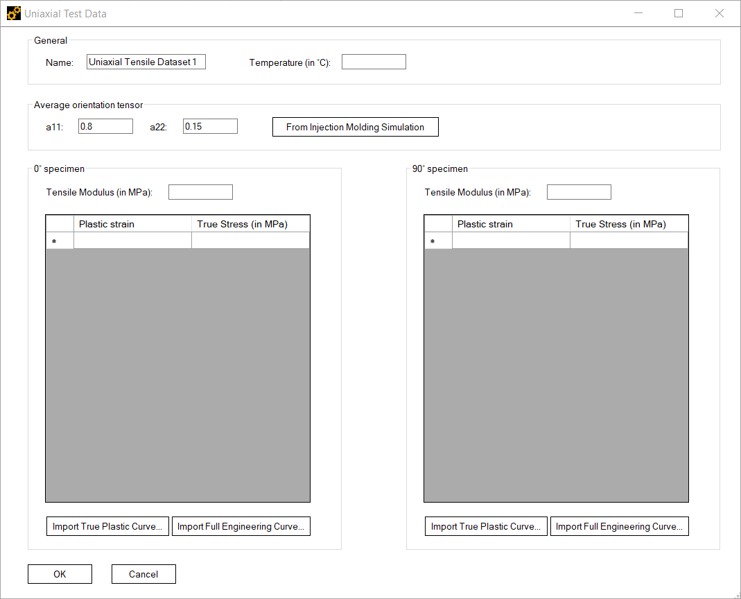
For each Dataset, you can click the   icon to open the dialog where you can review and edit the experimental data.

At a minimum, each Dataset should include the average orientation tensor and the Stress versus Plastic Strain curve of the specimens in the 0° and 90° degrees configuration. The tensile moduli are ignored by the Curve Fitting analysis.

The dialog has two columns, Plastic Strain and True Stress (in MPa). Click Import to import the stress-strain curves from a plain text file. The data file should be in character separated value (CSV) format with values delimited by spaces, tabs, or semicolons and dots used for decimal points. You can define multiple experimental Datasets, each at a different Temperature. In cases where only one experimental Dataset is specified, setting the temperature value is optional. Click   in the tool options to add another Dataset. Click   to remove it.

Figure 2.26: Uniaxial Dataset dialog

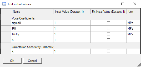
Fitting: Refer to B in Figure 2.25: Hill Plasticity Curve Fitting options. You can configure the plasticity model by specifying the Isotropic Hardening Model and the Hill Yield Model (see Fitting the Material Properties from Experimental Data for further details). You can also specify the initial values for the models coefficients. Click the Initial Values icon to open the dialog shown below.

Figure 2.27: Edit initial values dialog

Activating the check box in the adjacent column (Fix Initial Value) will fix the coefficient to the value specified in the Initial Value column.

Interpolation: (Refer to C in Figure 2.25: Hill Plasticity Curve Fitting options.) Use the Orientation Tensor Samples field to specify the number of sampling points when evaluating the Hill yield criterion over the relevant region of the orientation tensor space. (This region is highlighted in Figure 2.23: Samples in yellow are generated by symmetry considerations. See also the section on the Short Fiber Wizard.) Note that the values of the Hill yield are then automatically extended by symmetry to the entire orientation tensor space as described in Generated Material. You can also specify the options used afterwards to interpolate values. See also General Interpolation Library in the ACP User's Guide