Defining Frequency-Dependent Material Properties
HFSS provides several frequency-dependent material models. The Piecewise Linear and Frequency Dependent Data Points models apply to both the electric and magnetic properties of the material. However, they do not guarantee that the material satisfies causality conditions, and so they should only be used for frequency-domain applications.
The Debye and Djordjevic-Sarkar models apply only to the electrical properties of dielectric materials. These models satisfy the Kramers-Kronig conditions for causality, and so are preferred for applications (such as TDR or Full-Wave Spice) where time-domain results are needed. The Design Settings also include an automatic Djordjevic-Sarkar model to ensure causal solutions when solving frequency sweeps for simple constant material properties.
In HFSS, you can assign conductivity either directly as bulk conductivity, or as a loss tangent. This provides flexibility, but you should only provide the loss once. The solver uses the loss values just as they are entered.
Assigning Frequency-Dependent Properties
- From the Select Definition window, select a material and click View/Edit Material.
- Click Set Frequency Dependency.
The Frequency Dependent Material Setup Option dialog box appears.
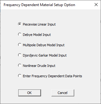
The options are:
- Piecewise Linear Input – defines the material property values as a restricted form of piecewise linear model with exactly 3 segments (flat, linear, flat). You specify the property's values at an upper and lower corner frequency. Between these corner frequencies, HFSS linearly interpolates the material properties; above and below the corner frequencies, HFSS extrapolates the property values. This dataset can be modified with additional points if desired.
- Debye Model Input – a single-pole model for the frequency response of a lossy dielectric material. In some materials, up to about a 10-GHz limit, ion and dipole polarization dominate and a single pole Debye model is adequate. HFSS allows you to specify an upper and lower measurement frequency, and the loss tangent and relative permittivity values at these frequencies. You may optionally enter the permittivity at optical frequency, the DC conductivity, and a constant relative permeability.
- Multipole Debye Model Input – allows you to provide the data of relative permittivity and loss tangent versus frequency. Based on this data, the software dynamically generates frequency-dependent expressions for relative permittivity and loss tangent through the Multipole Debye Model. The input dialog plots these expressions together with your input data through the linear interpolations. The generated expressions provide the new value for the material properties of relative permittivity and loss tangent. Both the expressions and data triples can be saved and reloaded.
- Djordjevic-Sarkar Model Input – for low-loss dielectric materials (particularly FR-4) commonly used in printed circuit boards and packages. In effect, it uses an infinite distribution of poles to model the frequency response, and in particular the nearly constant loss tangent, of these materials. This allows you to enter the relative permittivity and loss tangent at a single measurement frequency. You may optionally enter the relative permittivity and conductivity at DC.
- Nonlinear Drude Input – Drude materials are now supported by the transient solvers, producing plasma density data within the material domains. This means that plasma density plots can be produced.
- Enter Frequency Dependent Data Points – allows you to enter, import or edit frequency dependent data sets for each material property. Any number of data points may be entered. This is an arbitrary piecewise linear model.
- Select the input type and click OK.
An input type-specific dialog box appears, based on your selection.
Piecewise Linear Frequency Dependent Material Input, Debye Model Input, and Djordjevic-Sarkar Model Input remember the values previously used and also include plots to show the property curves in real time as changes to the input are made. Input values for each are saved as material attached data for the material being edited. These data items are saved with materials when they are written into a project file or exported to a material library. Note that when a frequency-dependent setup method is used and the values are pre-populated with saved data, the dialog box title will have "(Update)" appended.
After you have entered the data for your selection, you return to the View/Edit Material window. New default function names appear in the material property text boxes. HFSS automatically creates a dataset for each material property. Based on a varying property’s dataset, HFSS can interpolate the property’s values at the desired frequencies during solution generation.
To modify the dataset with additional points, see Editing Datasets.
Neither the piecewise nor the loss model asks for frequency-dependent conductivity because the constant sigma represents DC loss and the frequency-dependent loss tangent represents polarization losses.
Frequency Dependence Visualization
When you view or edit material properties, it is important to have a sense of how properties may vary with frequency. Frequency-dependent properties come in a variety of forms, ultimately resulting in some value expression or dataset. Plots of properties as a function of frequency are available through the View/Edit Materials window.
To view the plot:
- From the Select Definition window, select a material and click View/Edit Material.
- Right-click a property (for example, relative permittivity or dielectric loss tangent), and select View Property vs. Frequency.
The Frequency-Dependent Property Viewer appears, displaying the plot.
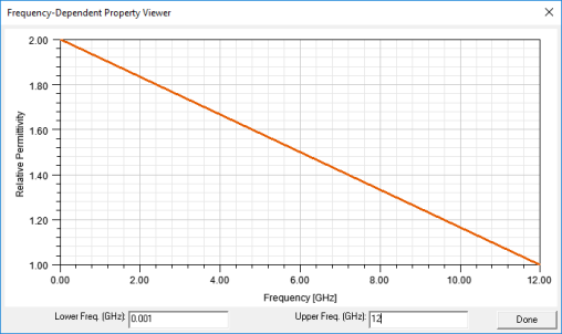
The window contains boxes where you can edit the frequency range for the plot. If the property was set by one of the nonlinear frequency setup methods, the frequency range will be derived from the data for that method, and edits to the lower/upper frequencies are not saved. Otherwise, the frequency range lower/upper frequency limit defaults are stored in the registry, and are updated if you modify the values. If values are not yet stored in the registry, the range defaults to 1MHz-10GHz. Note that the View Property vs. Frequency menu option is not displayed for choice properties because frequency-dependence doesn’t apply to those.
Saved Input Data Invalidation For Frequency-Dependent Setup
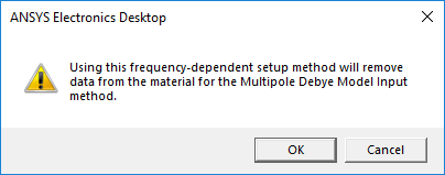
You will be prompted with a warning in two circumstances:
- Data associated with one of the frequency-dependent setup methods is attached to the material definition, and a property which would be set by this method is modified.
- Data associated with one of the frequency-dependent setup methods is attached to the material definition, and a different setup method is subsequently used.
You can choose OK to continue with the edit and remove the invalidated setup data, or choose Cancel to discard any changes.