General Multipaction Analysis Process
The process flow for running Multipaction Analysis follows:
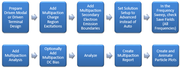
If you want to creation particle animations, you must select the Charge distribution option in the Multipaction Analysis setup to output particle and geometry mesh information.
Prepare a Driven Modal or Driven Terminal Design
As stated above, a multipaction analysis requires the time-harmonic fields being saved for a driven-terminal or driven-modal solution. Therefore, the multipaction setup and associated boundary conditions apply only to these types of HFSS projects. Other solution types, such as transient, eigenmode, characteristic mode, and SBR+, do not support the multipaction analysis. In addition, a multipaction simulation currently does not support renormalization or deembedding of ports.
Add Multipaction Charge Region Excitations
In HFSS Multipaction, charges are added to the simulation domain as excitations. A Multipaction Charge Region consists of either multiple objects or multiple faces, depending on whether the Selection Mode is Objects or Faces.
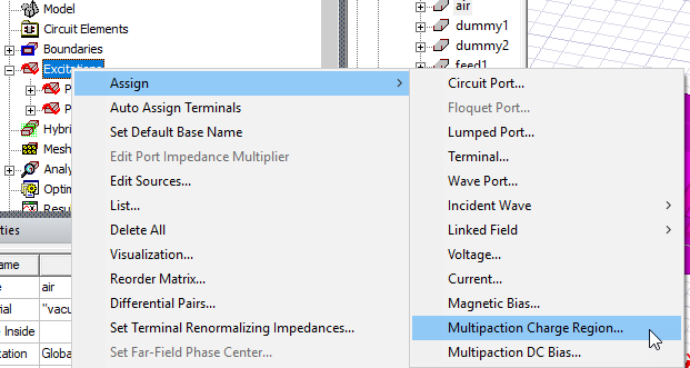
This opens the Multipaction Charge Region dialog box.
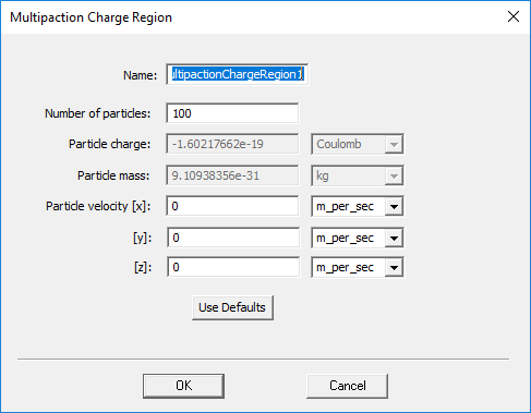
For each charge region, we can specify the number of electrons and their initial velocities. It is not necessary to seed charges in the entire simulation domain if the regions prone to multipaction can be easily identified, such as small gaps, coaxial feeds, parallel plates, and regions with strong fields. The simulation time can be significantly reduced by seeding charges only in critical regions.
The statistical variation of multipaction simulation can be reduced by using more particles, but the simulation time will increase as well. Moreover, using too few particles (less than 1000 for all charge regions) will introduce noises to the results and may trigger an early termination of the simulation.
Adding Multipaction Secondary Electron Emission (SEE) Boundaries
The Multipaction SEE boundaries should be added to vacuum-material interfaces where secondary electrons will be generated. Typically, those interfaces are associated with PEC, impedance, or finite-conductivity boundaries in electromagnetic simulation. If a Solve Inside object contacts the vacuum region, you should add SEE boundaries on their interface to avoid charged particles penetrating the object.
Charged particles will be entirely absorbed by surfaces in contact with vacuum but not covered by SEE boundaries. For example, port faces should not be covered by SEE boundaries because charged particles should be allowed to leave the simulation domain through ports.
Select the faces or objects to which you want to assign SEE boundaries, right-click on Boundaries in the Project Manager, and select Assign> Multipaction SEE... This command opens the Multipaction SEE dialog box:
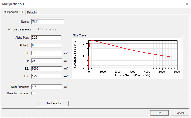
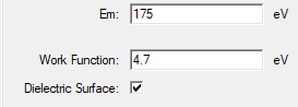
The secondary emission yield (SEY) depends on the impacting energy of the primary electron. We adopt an enhanced Vaughan model where the SEY curve will fall exactly on the low and high cutoff energies E1 and E2, where SEY is equal to 1. SEY reaches the maximum AlphaMax for an energy Em in between E1 and E2. For low-energy primary electrons, SEY is equal to Alpha0 when the impacting energy is between 0 and E0. The work function is needed for calculating the energy of secondary electron emission by the Chung-Everhart distribution. All energies related to the SEE boundary are measured in electron volts (eV). You must check the Dielectric Surface checkbox for an insulator-vacuum interface, which allows the accumulation of positive surface charges after secondary electrons leave the interface, or the accumulation of negative surface charges after the interface absorbs primary electrons.