Adding a Multipaction Setup

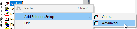
At least one charge region and one SEE boundary must exist before you can add a Multipaction Analysis. To add a Multipaction Analysis, you must add a Solution Setup and a Frequency Sweep. You then add the Multipaction Setup to the Sweep. When you add the Solution Setup to an Analysis in HFSS, select Advanced instead of Auto.

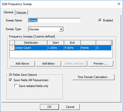
The frequencies specified in the frequency sweep will be reused for setting up the multicarrier signal for a multipaction analysis. You must select the Save Fields (All Frequencies) checkbox while editing the frequency sweep, otherwise Add Multipaction Analysis will be grayed out on the menu. There will be no multipaction if there is no time-harmonic field to sway the charged particles in the simulation domain.

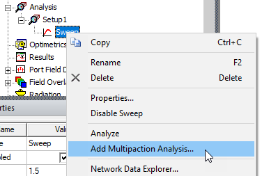
Once the above procedures are completed, you can right-click the frequency sweep and select Add Multipaction Analysis...

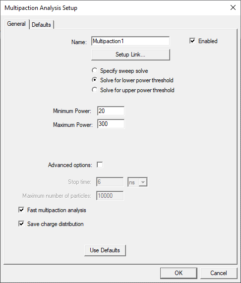
This opens the Multipaction Analysis Setup dialog box.

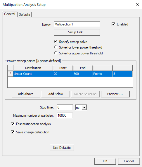
The Solve for lower power threshold button allows automatic determination of the lower power threshold. It is the power threshold where the breakdown status transits from no multipaction to multipaction with increasing input power. Similarly, the Solve for upper power threshold button allows automatic determination of the upper power threshold. It is the power threshold where the breakdown status transits from multipaction to no multipaction with increasing input power.

Given the power range provided by the user, the software determines which power multiplier to simulate next based on previous multipaction history, instead of reading preset power multipliers from a table. By default, the advanced options are off. The lowest power threshold is found using a stop time ranging from 80 to 120 RF cycles and no more than twice the initial number of particles. The default settings can be overridden by checking advanced options if users prefer to set up the parameters by themselves

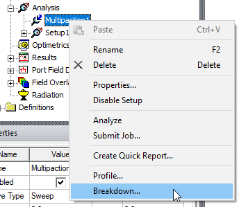
While the automatic simulation is running, you can check the breakdown status of simulated power multipliers by clicking Breakdown... under the multipaction setup shortcut menu.

This opens a Solutions dialog box with a Multipaction tab that provides Power and Breakdown information as follows:

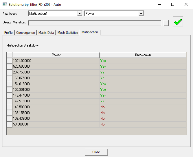
When the Auto Solve converges, there will be a message showing the lowest multipaction power threshold in the Message Manager window.

If the Auto Solve does not converge, it means the structure is free of multipaction for given geometry, material, and simulation setups.

Whether you choose Sweep Solve or Automatic Solve, you have to click Setup Link… to link the multipaction analysis with a frequency sweep before running the multipaction simulation.

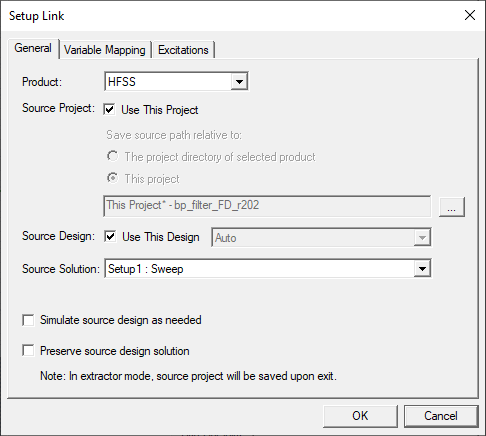
By default, the link points to the current project, design, and sweep. After setting up the source, click the Excitations tab so you can specify the excitations or the DC bias fields for the multipaction analysis.

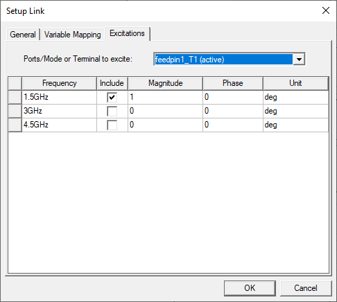
You must include at least one terminal with a positive magnitude. The input signal for each mode or terminal is a linear combination of multi-carrier signals multiplied by the square root of the power multiplier:

where is the port voltage of the i-th carrier with one-watt input power in driven-modal solutions. For driven-terminal solutions, the input power of a port is not one-watt. Therefore, scaling must be done before applying the above formulation for calculating the port voltage.

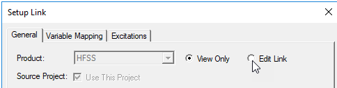
After setting up the excitations, press OK to complete the link setup. Afterward, you can only edit the Setup Link if you click Edit Link. Otherwise, the Setup Link dialog box will be in read-only mode.

The second step in the Multipaction Analysis dialog box, if you have selected Sweep solve, is to set up the stop criteria by a stop time and the maximum number of particles.

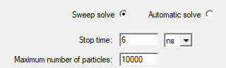
The multipaction simulation will be terminated according to the stop time, which is usually set to 20 cycles of the lowest frequency of the multicarrier signal. The simulation also terminates when the number of particles reaches zero or exceeds the maximum number of particles.

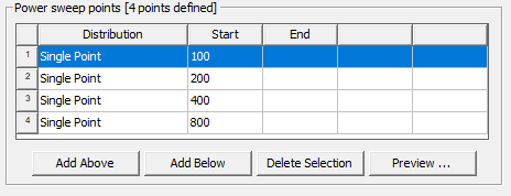
The third step for Sweep solve is to specify power sweep points or multipliers for scaling the power of each port mode or terminal voltage. Each mode in a driven-modal design, or each terminal in a driven-terminal design has one-watt input power. When there is only one mode or one terminal active, the power multiplier is essentially the input power of the multipaction analysis.

The fourth step for both Sweep solve and Automatic solve is to select whether the multipaction analysis type will be fast or not. The fast simulation is less compute-intensive but also less accurate when the structure to be analyzed has complex geometry and fine details. However, our tests show that the fast simulation is satisfactory for most applications.

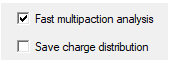
The last step is to choose whether to write out Charge distribution and model geometry. This data can be displayed as particle overlays and animations in Electronics Desktop.

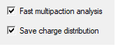
Saving charge distribution involves writing to a hard drive and will slow down the simulation. If the goal is to predict the multipaction power threshold, the overhead can be avoided by unchecking the option.

The model and particle files (*.vtu) will be written to a directory at the same level as the HFSS project:

Optional Multipaction DC Bias

It is optional to set up DC electric or magnetic bias fields for a multipaction analysis.

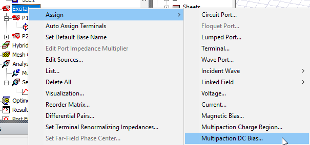
This opens the Multipaction DC Bias dialog box.

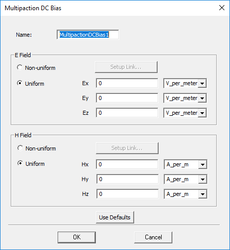
The type of bias can be either uniform or nonuniform. For a uniform bias, the field values are the same throughout the entire simulation domain. The non-uniform bias fields are specified through Maxwell near field links.