


Whether you are beginning a new simulation or modifying an existing one, it is a good idea to ensure that your simulation parameters are set exactly the way you want before you start processing. Once you Start a Simulation and begin processing, you cannot go back and change the settings without losing the simulation results that have been created.
Setting simulation parameters involves setting simulation-wide values as well as parameters specific to SPH, geometries, materials, inlets and outlets, and more. To make the setup of multiple similar items quicker, you many also choose to duplicate already-setup items, or remove many similar items at one time.
You set simulation-wide parameters when you want to change the default values provided by FreeFlow to affect your whole simulation. Simulation-wide parameters are settings that can include:
Study items, which include setting the simulation title and customer name.
Physics items, which include setting how you want gravity applied and enabling Thermal model.
Modules items, which include SPH Density Monitor and SPH Boundary Interaction Statistics, for example.
Domain Settings items, which include defining the simulation coordinate limits and settings and optional periodic domain.
Solver items, which include setting simulation time length, and certain data collection times.
Simulation-wide parameters are set by first selecting the Study, Physics, Modules, Domain Settings, and Solver sections in the Data panel and then editing the results in the Data Editors panel.
These values can be set at any time before you begin processing your simulation. However, it is recommended that at least the Physics and Modules settings be made first as your selections there may affect other settings later on.
Keep in mind that there are minimum requirements for processing a simulation.
FreeFlow comes preset with default values that you can use right away without modification if you choose. However, the minimum requirements for processing a simulation include setting up each of the following items:
One Inlet.
Mass Flow Rate or Velocity.
What would you like to learn about?
Use the figures and table below to help you understand the various Study parameters you can set for a simulation project.
Note: Unlike most other setup parameters, you are able to chance your Study parameters at any time, even during active processing. (See also I cannot change my setup parameters during processing.)
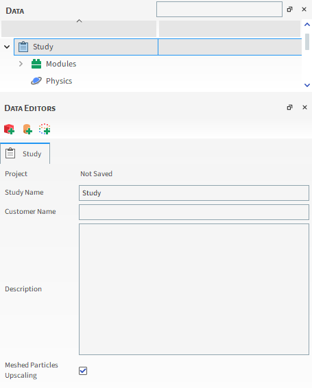
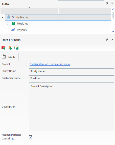
Table 3.1: Study Parameter Options
| Setting | Description | Range |
|---|---|---|
| Project | When the project is saved, this lists the full path for the .FreeFlow project file in hyperlink form (Figure 3.4: Study Parameters in the Data Editors panel (Saved project with information entered)). If the project has not yet been saved, "Not Saved" will be displayed (Figure 3.3: Study Parameters in the Data Editors panel (Default, unsaved project)). | Path automatically provided |
| Study Name | Name of the simulation you are working on. For example, "Dishwasher". Note: The Study entity on the Data panel will be renamed with what you enter here (Figure 3.4: Study Parameters in the Data Editors panel (Saved project with information entered)). | No limit |
| Customer Name | Name of the customer for whom you are doing the simulation. | No limit |
| Description | Description of the simulation | No limit |
What would you like to do?
See Also:
The FreeFlow Physics parameters include simulation-wide settings that affect how the components are calculated. These include settings affecting gravity and the separate settings that enable Thermal Modeling.
ABOUT PHYSICS PARAMETERS
Read below to understand the Physics Parameters that can be set for a simulation project.
GRAVITY PARAMETERS
The following Table contains a description of each option in the Physics parameters panel.
Table 3.2: Physics Parameter Options
| Setting | Description | Range |
|---|---|---|
| Gravity | ||
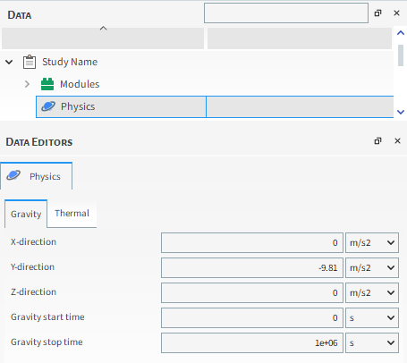
| X Direction | Used to change the direction that gravity affects SPH elements
and free boundaries, this is the amount of acceleration applied in
the X direction during the simulation. Tip: When prescribing movements, it can be easier to align geometries with the global axes and then simulate gravity in the plane that represents downward forces. For example, if you had your equipment horizontally aligned with the X direction, you could then modify the Y and X components of gravity to simulate it as if it were inclined in the YX plane. | No limit |
| Y Direction | Used to change the direction that gravity affects SPH elements
and free boundaries, this is the amount of acceleration applied in
the Y direction during the simulation. Note: The default value is -9.81 m/s2, which accounts for the effect of gravity pointing in the downward Y direction only. | No limit |
| Z Direction | Used to change the direction that gravity affects SPH elements and free boundaries, this is the amount of acceleration applied in the Z direction during the simulation. | No limit |
| Gravity Start Time | The duration you want to wait before gravity components are activated. | Positive values |
| Gravity Stop Time | The duration you want to wait before gravity components are deactivated. | Positive values |
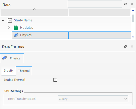
| Thermal | ||
| Enable Thermal | Makes possible the simulation of conductive heat transfer between
SPH elements and Walls. Enables convective heat transfer between SPH
elements and fluids when coupled with Ansys Fluent. See also Enable Thermal Modeling | On or Off |
| SPH Settings (Thermal) | ||
| Heat Transfer Model | When Enable Thermal is selected, this is the type of model used
to calculate heat transfer for SPH elements. Unless you have enabled a custom external module that defines a different Heat transfer Model, only the default, Cleary model, will be used. | Cleary Note: This setting is considered to be exclusive so if you have one or more external Module that are able to override this model, you must have only one such Module enabled within your simulation project. |
What would you like to do?
See Also:
When you enable a Module in FreeFlow, you are choosing to add in custom, discrete features and/or functionality within your project. Depending upon the type of Module you enable and what it does, there may be additional settings that affect other areas of your FreeFlow project setup.
Use this topic to understand more about Module parameters and how setting them affects your project.
Tip: To learn more about the different types of FreeFlow Modules and where you obtain them, refer to the topic About FreeFlow Modules.
ABOUT FreeFlow MODULES PARAMETERS
Cover the basics about enabling modules, setting modules, and other important informations.
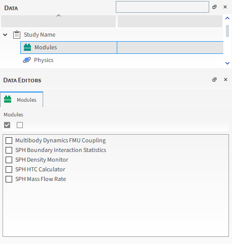
Because the default state for most Modules is disabled, it becomes very important for you to ensure that you have enabled the Modules and options you want prior to setting up the rest of your simulation. This is done by selecting the main Modules entity in the Data panel and then enabling the checkbox for the module you want to use in the Data Editors panel (Figure 3.7: Modules Available by Default in FreeFlow).
Important: Only embedded Modules andexternal Modules that you have already installed will appear on the list. (See also Install an External Module.)
In addition, because it is possible that turning on a Module will add or change options presented in other parts of the FreeFlow setup, it is recommended that turning on the Modules and options you want is one of the very first steps you take when setting up your project.
Tip: If you have similar projects that you set up regularly, using a script to record and then play back your Module configuration steps can save you from having to repeat these steps on future projects. (See also About Creating and Using PrePost Scripts.)
Note: Enabling more than one Module at once can cause some parameters to be shared across Modules. (See also Recognize Shared Parameters with Asterisks (*).)
Once enabled, many types of Modules have parameters that you can define. Depending upon the type of Module and what it does, the settings can be in any of the following combinations.
Module Enables no Additional Settings
For these types of Modules, once you enable the Module itself, the functionality will be applied without any additional actions from you.
An example of this kind of Module is the SPH Density Monitor Module.
Tip: You will know that a Module has no additional settings when you select it from the Data panel, and find no settings on the Module's Data Editors panel, and its Info tab says "Module does not affect any simulation entity."
Module Enables Additional Settings
For these types of Modules, once you enable the Module itself, there are one or more additional settings in one or both of the following locations:
On the Module's Data Editors panel
For these types of Modules, there are one or more additional settings to be made on the Data Editors panel for the Module.
An example of this kind of Module is the SPH HTC Calculator Module.
Elsewhere in the FreeFlow setup
For these types of Modules, there are one or more additional settings to be made in (or have otherwise been affected by) other locations of the FreeFlow UI. These may require additional setup steps for the Module in those other locations.
Example Module to be selected.
Tip: You will know that a Module has other settings in (or is otherwise affecting) other parts of the FreeFlow setup when you select it from the Data panel and then from the Data Editors panel, see that its Info tab has information next to the Affected Simulation Entities label. You can then use that information to discover where else in the FreeFlow setup Module-specific settings might need to be applied.
Learn more about where and when you might define parameters for your Modules.
About the Main Tab for Modules
Once enabled, some types of Modules will have additional settings on the Module's main tab in the Data Editors panel. To learn if there are additional, Module-specific settings that affect other parts of your FreeFlow project setup, you can view the information on the Info tab.
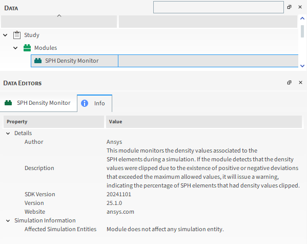
About the Info Tab for Modules
The Info tab on individual Modules describe the Author and Version details for the Module, and lists what other entities in the FreeFlow UI are affected by enabling that particular Module.
For example, the Info tab for the SPH Density Monitor describes three places in the FreeFlow UI affected by that module.
This information can help you verify that the parameters in those locations are set correctly for the feature enabled by the module.
Module-Specific Settings on Other FreeFlow UI Locations
Once enabled, some Modules will cause other areas of the FreeFlow UI to have additional settings specific to that Module, or will cause other changes, such as model overrides. These kinds of changes and additional settings are unique to each Module, so the best way to determine what other settings might be required for your Module is to view the Affected Simulation Entities information on the Info tab. More about Affected Simulation Entities.
Once you understand what other parts of the UI are affected, you can then be sure to verify the Module-specific settings in those areas when setting up the rest of your project.
Tip: To learn more about what specific FreeFlow UI settings and options Modules can affect, refer to the FreeFlow Simulation Entities that can be Affected by Modules topic.
What would you like to do?
Learn about SPH Boundary Interaction Statistics Module
Learn about SPH Density Monitor Module
Learn about SPH HTC Calculator Module
Learn about SPH Mass Flow Rate Module
See Also:
Geometries are the physical boundaries that make up the components that are going to be simulated in FreeFlow. They can be geometries that you import from various CAD programs, or from Ansys Fluent or Ansys Motion setup files, and also surfaces created directly in FreeFlow.
You can add as many individual geometry components as you want to your simulation in any combination you desire.
However, if you are using a fluid inlet to release SPH elements into your simulation (see also About Adding and Editing Inlets and Outlets), before you are able to process the simulation, you must have a minimum of at least one inlet set up. If you are using a Volumetric Inlet, a simulation can be set up with no geometries in it.
Once you add the geometries you want, you can then change the parameters to achieve the behavior you want. The parameters you change can include the size, shape, and behavior of the default geometries included within FreeFlow, or special movements of the geometries you have imported, such as gates that lift or turn, for example.
At any point, you can see how your geometries look in a 3D View (see also Create and Modify a 3D View.)
What would you like to do?
See Also:
There are two categories of geometries that you can add to your simulation: surfaces and walls; additionally FreeFlow offers you the option to use templates that can combine both types of geometries.
Surfaces are geometries that allow for the passage of SPH elements. They can be set up as inlets, outlets, or as flow measuring surfaces. They can also delimit regions in space that can be filled with fluid. If you want a geometry to act as an barrier that can stop fluid from flowing through it, this geometry must be set up as a wall.
Important: If you want to use a surface as an Inlet or an Outlet, the surface must be planar (i.e. it should be contained into a single plane).
Tip: Surfaces have a Normal Direction property, which indicates the direction of injection and removal for inlets and outlets and, also, the sign of flow measurements. In FreeFlow, there is an Invert Normal option, which inverts the normal of the surface and, as a consequence, inverts the directions for inlets/outlets and the flow measurements.
In FreeFlow, geometries can be created or imported from external CAD/CAE softwares. The following options to create or import geometries are available (through the Geometry option on the Data panel). See Geometry Options Available in FreeFlow.
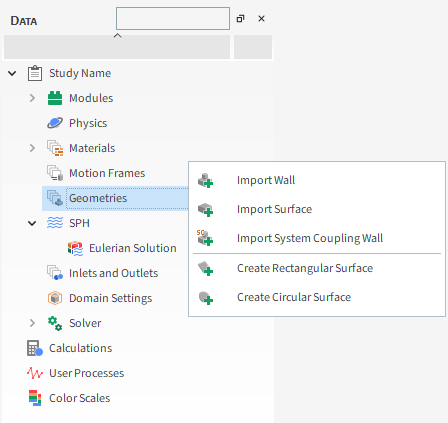
Import Wall: Allows you to import a geometry that will act as a Wall. (See also Import Wall or Surface Geometries)
Import Surface: allows you to import a geometry that will act as a Surface. (See also Import Wall or Surface Geometries)
Import System Coupling Wall: allows you to import a geometry that will act as a Surface. (See also Import System Coupling Wall)
Create Rectangular Surface: allows you to create a rectangular geometry inside FreeFlow that will act as a Surface. (See also Add New Circular and Rectangular Surfaces)
Create Circular Surface: allows you to create a circular geometry inside FreeFlow that will act as a Surface. (See also Add New Circular and Rectangular Surfaces)
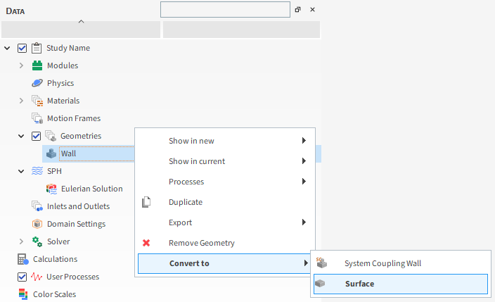
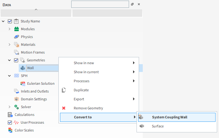
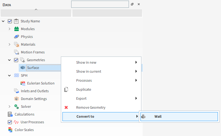
CONVERSIONS OF WALLS AND SURFACES
In addition to the possibility to import Walls or Surfaces into your project, you can also convert Walls into Surfaces and Imported Surfaces into Walls.
To do so, right-click the choose geometry, in the Data Panel, and then go to the option Convert to, as illustrated in the Figures below:
What would you like to do?
ADD NEW CIRCULAR AND RECTANGULAR SURFACES
You can create rectangular and circular planar surfaces inside FreeFlow, eliminating the need of importing these geometries from an external CAD software. Since these geometries will act as an surface, you can use them to set inlets, outlets (see also Add and Edit Inlets and Outlets) and to perform flow measurements.
To create these surfaces, do all of the following:
From the Data panel, click Geometries, and then from the Data Editors panel, click the Create Rectangular Surface or Create Circular Surface button. A new Rectangular/Circular Surface component appears under Geometries in the Data panel.
Tip: You may also access this functionality from the right-click menu on the Data panel.
From the Data panel, click the Rectangular/Circular component you just added and then from the Data Editors panel, on the main Rectangular/Circular Surface tab, enter the Name you want. You can also edit the properties listed in the table below.
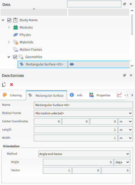
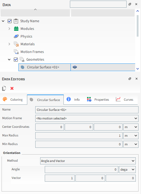
Table 1: Options available when creating a Rectangular or Circular Surface
|
Setting |
Description |
Range |
|---|---|---|
|
Name |
Enables you to specify a unique identifier for the geometry component |
99 character limit |
|
Motion Frame |
Enables you to select which Motion Frame you want assigned to the geometry. (See also About Creating and Applying Motion Frames). |
Automatically provided |
|
Center Coordinates |
Enables you to define X, Y and Z coordinates of the center of the geometry. |
Any value |
|
Max Radius (Circular Surface Only) |
Defines the radius of external limit of the circular geometry. |
Positive Values |
|
Min Radius (Circular Surface Only) |
Defines the radius of internal limit of the circular geometry. |
Positive Values |
|
Lenght (Rectangular Surface Only) |
Defines the transverse dimension of the rectangular geometry. |
Positive Values |
|
Width (Rectangular Surface Only) |
Defines the longitudinal dimension of the rectangular geometry. |
Positive Values |
|
Method |
Enables you to select how you want to define the orientation of the geometry. Specifically:
|
Angles; Angle and Vector; Basis Vectors |
|
Method Angles | ||
|
Order |
When Angles is selected for Orientation, this defines the order in which the three Rotation fields will be applied. |
XYZ; ZXY; YXZ; YZX; ZXY; ZYX |
|
Local Angles |
When Angles is selected for Orientation, this defines what coordinate system will be used as a basis for the angle specified. Specifically:
|
Turns on or off |
|
Rotation |
When Angles is selected for Orientation, this is the degree of cube rotation in each of the three directions specified by the Order provided. |
Any value |
|
Method Angle and Vector | ||
|
Angle |
When Angle and Vector is selected for Orientation, this is the angle the cube will rotate around the Vector defined. |
Any value |
|
Vector |
When Angle and Vector is selected for Orientation, this is the X, Y, and Z components that define the vector around which the cube will rotate, using the Angle defined. |
No limit but the values entered will be normalized |
|
Method Basis Vectors | ||
|
X direction |
When Basis Vectors is selected for Orientation, this is the coordinate values defining the first of three directional vectors that together define the final orientation of the cube. Tip: To ensure correct results, make sure you define this vector as orthogonal (perpendicular) to the other two vectors. |
No limit but the values entered will be normalized |
|
Y direction |
When Basis Vectors is selected for Orientation, this is the coordinate values defining the second of three directional vectors that together define the final orientation of the cube. Tip: To ensure correct results, make sure you define this vector as orthogonal (perpendicular) to the other two vectors. |
No limit but the values entered will be normalized |
|
Z direction |
When Basis Vectors is selected for Orientation, this is the coordinate values defining the third of three directional vectors that together define the final orientation of the cube. Tip: To ensure correct results, make sure you define this vector as orthogonal (perpendicular) to the other two vectors. |
No limit but the values entered will be normalized |
What would you like to do?
IMPORT WALL OR SURFACE GEOMETRIES
All geometries that are not rectangular or circular, or have a template inside FreeFlow (such as conveyors), need to be imported. Imported geometries can be set up as both wall and surface. When imported as surfaces, the geometry can be used for flow measurements, as an inlet or an outlet (if planar). Importing geometry as walls allows for them to be used for additional calculations (such as surface wear or heat conduction).
FreeFlow supports importing geometries with the following file extensions: STL, DXF, XGL, CAS, CAS.GZ, CAS.H5, MSH, FMU, or DFG.
To import these surfaces, do all of the following:
From the Data panel, click Geometries, and then from the Data Editors panel, click the Import Wall or Import Surface button.
Tip: You may also access this functionality from the right-click menu on the Data panel.
Select the file that you want to import into FreeFlow and click Open.
Tip: To save time on larger projects, you may also want to import multiple components at once by multi-selecting several files on the Select file to import dialog.
Select the file that you want to import into FreeFlow and click Open.
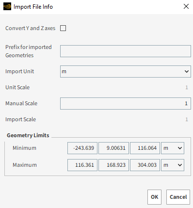
After choosing which file(s) you want to import, you are asked to define several options that enable you to determine the scale and unit of the imported file(s) (Figure 3.15: Import File Info Dialog). In addition, you can either choose to import the component names as they are by leaving the Prefix for imported Geometries blank, or you can add custom text to prefix the component name with whatever you like.
Imported geometry components may be replaced with a different geometry file prior to processing. (See also Replace an Imported Geometry File.)
Note: If you want to use a geometry for flow measurements or other post-processing analysis, it must be imported into FreeFlow before the simulation has started. In post-processing FreeFlow is not able to import a geometry without needing to restart the simulation.
Use the figure and table below to understand the various import parameters you can set for your imported geometries and then use the procedures that follow to learn about how to add geometry components to your simulation setup.
Table 3.3: Import Options Displayed in the FreeFlow Dialog
Setting Description Range Convert Y and Z axes
Selecting this option will change the axis of the imported geometry.
Turns on or off
Prefix for imported Geometries
When cleared (blank), the name of the imported file will be displayed in the Geometries list. When defined, this additional name will be displayed directly before the imported name in the Geometries list. If the geometry contains multiple components, each component will have this same prefix followed by the (unique) imported name of the file.
99 character limit
Import Unit
Enables you to change the units of the imported geometry.
Various units of length
Unit Scale
Displays the unit scale based upon the Import Unit set. For example, if Import Unit is left as the default value, the Unit Scale will be 1.
Automatically determined
Manual Scale
Enables you to manually adjust the scale by any factor you want. Leaving the value at 1 will have no additional affect upon the scale.
All values
Import Scale
Displays the final import scale based upon the Manual Scale and Import Unit values set. For example, if both those options are left as the default values, the Import Scale will be 1.
Automatically determined
Geometry Limits
Minimum
The coordinates (in X Y Z format) of the lowest points geometry triangles are drawn.
No limit
Maximum
The coordinates (in X Y Z format) of the highest points geometry triangles are drawn.
No limit
Importing a Geometry as a Surface
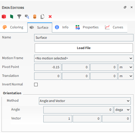
Use the figure and table below to understand the various import parameters you can set for a geometry that was imported as a surface.
Prior to processing, Geometry components may be replaced with a different geometry file, (see also Replace an Imported Geometry File), and have a Motion Frame assigned to them (see also Apply a Motion Frame to an Imported Geometry.)
Table 3.4: Options Available for Geometries Imported as Surfaces
Setting Description Entry Name
Enables you to specify a unique identifier for the geometry component
99 character limit
Motion Frame
Enables you to select which Motion Frame you want assigned to the geometry. (See also About Creating and Applying Motion Frames.)
Automatically provided
Pivot Point
The coordinate location of the point around which the surface will pivot, as specified in the X, Y, and Z directions.
Note: In the calculation order, the rotation is calculated before the translation. In this way, the Pivot Point presented in the UI does not include the translation values, therefore to obtain the real value, it is necessary to sum the pivot point values with the translation values.
No limit
Translation
Enables you to move the geometry in the X, Y and Z directions
Zero or Positive Values
Orientation
Enables you to select how you want to define the orientation of the geometry. Specifically:
Angles enables you to define angles of rotation in three directions, the order of which you can also specify.
Angle and Vector enables you define one vector and one angle of rotation around it.
Basis Vectors enables you to define the X, Y, and Z directions of the geometry local basis.
Angles; Angle and Vector; Basis Vectors
Orientation Angles
Order
When Angles is selected for Orientation, this defines the order in which the three Rotation text fields will be applied.
XYZ; ZXY; YXZ; YZX; ZXY; ZYX
Local Angles
When Angles is selected for Orientation, this defines what coordinate system will be used as a basis for the angle specified. Specifically:
When enabled, the angle will be based on the local coordinate system.
When cleared, the angle will be based on the global coordinate system.
Turns on or off
Rotation
When Angles is selected for Orientation, this is the degree of cube rotation in each of the three directions specified by the Order provided.
Any value
Orientation Angle and Vector
Angle
When Angle and Vector is selected for Orientation, this is the angle the cube will rotate around the Vector defined.
Any value
Vector
When Angle and Vector is selected for Orientation, this is the X, Y, and Z components that define the vector around which the cube will rotate, using the Angle defined.
No limit but the values entered will be normalized
Orientation Basis Vectors
X direction
When Basis Vectors is selected for Orientation, this is the coordinate values defining the first of three directional vectors that together define the final orientation of the cube.
Tip: To ensure correct results, make sure you define this vector as orthogonal (perpendicular) to the other two vectors.
No limit but the values entered will be normalized
Y direction
When Basis Vectors is selected for Orientation, this is the coordinate values defining the second of three directional vectors that together define the final orientation of the cube.
Tip: To ensure correct results, make sure you define this vector as orthogonal (perpendicular) to the other two vectors.
No limit but the values entered will be normalized
Z direction
When Basis Vectors is selected for Orientation, this is the coordinate values defining the third of three directional vectors that together define the final orientation of the cube.
Tip: To ensure correct results, make sure you define this vector as orthogonal (perpendicular) to the other two vectors.
No limit but the values entered will be normalized
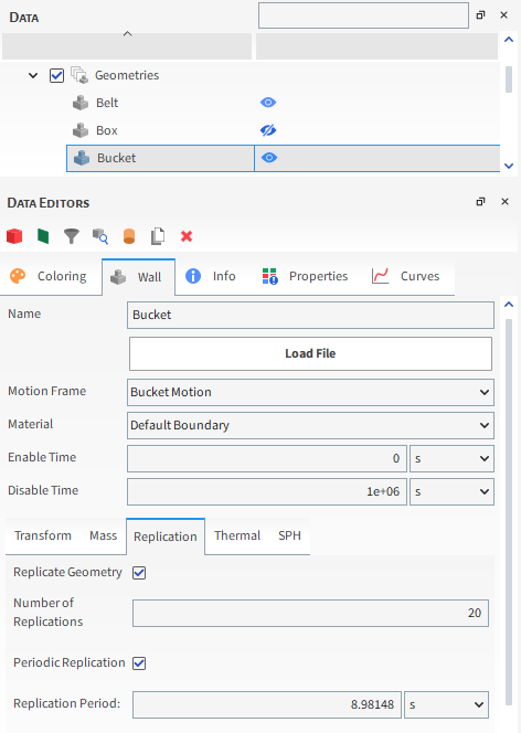
About Importing a Geometry as Wall
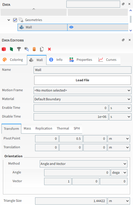
After you have imported a geometry as a wall, you can then edit the Geometry, Mass, Replication, Thermal and SPH parameters that define how the geometry behaves in the simulation.
Prior to processing, Geometry components may be replaced with a different geometry file, (see also Replace an Imported Geometry File), and have a Motion Frame assigned to them (see also Apply a Motion Frame to an Imported Geometry.)
After processing, Geometry components can be exported out of FreeFlow into an STL file, which is especially useful after the geometry surface has been modified by wear. (See also Export a Geometry Component to an STL File.)
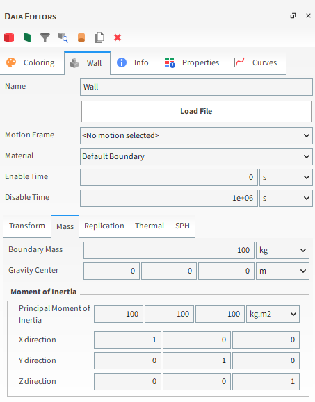
The mass settings are only useful when a Motion Frame with either Free Body Translation or Free Body Rotation has been applied to the geometry. This is to ensure that the component behaves correctly in terms of gravity and any additional (prescribed) force/moments effects, as well as interactions with SPH elements.
Tip: The Principal Moment of Inertia values can be determined in your CAD program.
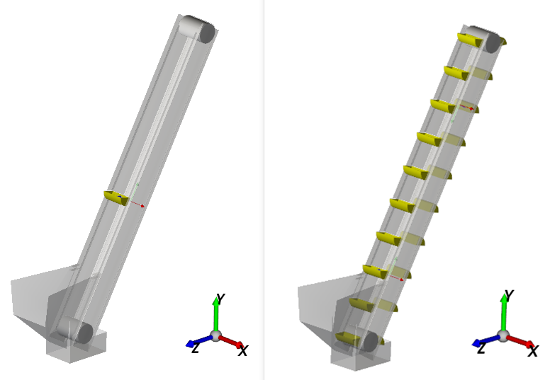
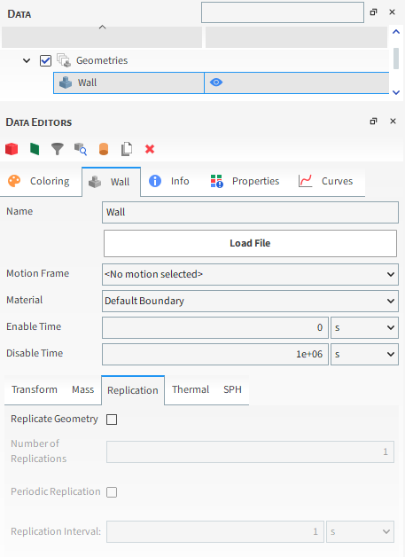
The replication settings, when coupled with Motion Frames and periodic motions, enable you to reproduce a geometry component at intervals along the path of the assigned motion. This can be useful for turning a single bucket into a full bucket elevator, as shown in the example below.
Replication can also be previewed in a Motion Preview window before processing the simulation. (See also Preview a Motion in 3D.)
Note: Geometry replication features are not compatible with free body motions. (See also About Creating and Applying Motion Frames.)
Modules Parameters
If you have enabled an external Modules that affects your Geometries settings, you might also have a separate Modules sub-tab with additional settings that you can define. Refer to the Module's documentation (if provided) for more information. (See also FreeFlow Simulation Entities that can be Affected by Modules.)
Note: None of the embedded FreeFlow Modules will activate the Modules Tab in Imported Wall Parameters.
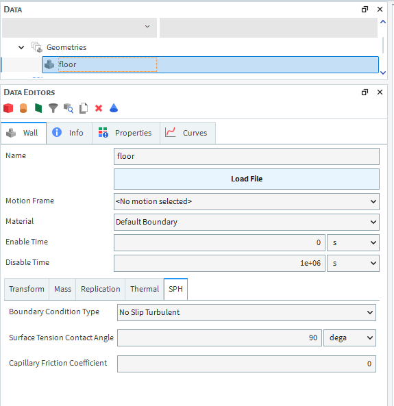
Use the following figures and table to understand the various Geometry, Mass, Wear, and Replication parameters that you can set for an imported geometry.
Table 3.5: Imported Wall Parameter Options (Geometry, Mass, Replication, Thermal and SPH)
Setting Description Range Name
Enables you to specify a unique identifier for the wall component.
No limit
Motion Frame
Enables you to select which Motion Frame you want assigned to the geometry. (See also About Creating and Applying Motion Frames.)
Automatically provided
Material
Defines the density and Young's Modulus of the wall component based upon the options you have set in the Materials list.
When Thermal Model is enabled (see also About Physics Parameters.), this also defines the specific heat and Poisson's ratio values, both of which are set in the Materials list.
List is based upon the Materials that have been defined
Enable Time
The time you want the geometry to start interacting with SPH elements during the simulation.
Tip: To have the geometry interact with SPH elements at simulation onset, keep Enable Time as zero (0).
Note: If you choose to use parametric expressions in this field, know that only the resulting value and not the variables and/or mathematical functions you enter will be retained in any project copies you save for restart purposes.
Positive values
Tip: Check the Status panel to ensure that any variables or mathematical functions you might use results in valid values. (See also Double-click the Status Panel to Jump to the Appropriate UI Location.)
Disable Time
The time you want the geometry to stop interacting with SPH elements during the simulation.
Tip: To have the geometry interact with SPH elements for the duration of the simulation, keep Disable Time as 1e+06 or the maximum length of your simulation.
Note: If you choose to use parametric expressions in this field, know that only the resulting value and not the variables and/or mathematical functions you enter will be retained in any project copies you save for restart purposes.
Positive values
Tip: Check the Status panel to ensure that any variables or mathematical functions you might use results in valid values. (See also Double-click the Status Panel to Jump to the Appropriate UI Location.)
Transform
Pivot Point
The coordinate location of the point around which the wall will pivot, as specified in the X, Y, and Z directions.
Note: When FreeFlow calculates the transformation of coordinates of walls/surfaces, the operation of rotating the geometry around the pivot point comes first, then the translation operation is applied on those rotated coordinates. As a consequence, the pivot point that is inputted in the UI is the position of the pivot point before the translation, while the pivot point that appears in the 3D view is the pivot point after the translation operation.
No limit
Translation
Enables you to move the geometry in the X, Y and Z directions.
Zero or Positive Values
Orientation
Enables you to select how you want to define the orientation of the wall shape. Specifically:
Angles enables you to define angles of rotation in three directions, the order of which you can also specify.
Angle and Vector enables you to define one vector and one angle of rotation around it.
Basis Vectors enables you to define the X, Y, and Z directions of the cube’s local basis.
Angles;
Angle and Vector;
Basis Vectors.
Orientation: Angle and Vector
Angle
When Angle and Vector is selected for Orientation, this is the angle the wall will rotate around the defined Vector.
Any value
Vector
When Angle and Vector is selected for Orientation, this is the X, Y, and Z components that define the vector around which the wall will rotate, using the defined Angle.
No limit but the values entered will be normalized
Orientation: Basis Vector
X direction
When Basis Vectors is selected for Orientation, this is the coordinate values defining the first of three directional vectors that together define the final orientation of the wall. Tip: To ensure correct results, make sure you define this vector as orthogonal (perpendicular) to the other two vectors.
No limit but, the values entered will be normalized
Y direction
When Basis Vectors is selected for Orientation, this is the coordinate values defining the second of three directional vectors that together define the final orientation of the wall. Tip: To ensure correct results, make sure you define this vector as orthogonal (perpendicular) to the other two vectors.
No limit but,the values will be normalized
Z direction
When Basis Vectors is selected for Orientation, this is the coordinate values defining the third of three directional vectors that together define the final orientation of the wall. Tip: To ensure correct results, make sure you define this vector as orthogonal (perpendicular) to the other two vectors.
No limit but,the values will be normalized
Orientation: Angles
Order
When Angles is selected for Orientation, this defines the order in which the three Rotation text fields will be applied.
XYZ;
ZXY;
YXZ;
YZX;
ZXY;
ZYX.
Local Angles
When Angles is selected for Orientation, this defines what coordinate system will be used as a basis for the angle specified. Specifically:
When enabled, the angle will be based on the local coordinate system.
When cleared, the x angle will be based on the global coordinate system.
Turns on or off
Rotation
When Angles is selected for Orientation, this is the degree of wall rotation in each of the three directions specified by the Order provided.
Any value
Triangle Size
Size of the triangular components into which the boundary is divided.
This value is used for refining the boundary mesh (this will not happen if the imported Triangle Size is already finer than this value).
Positive values
Mass
Boundary Mass
When Free Body Translation or Free Body Rotation are defined for the Motion Frame applied to this geometry, this is the mass of the geometry.
Positive values
Gravity Center
When Free Body Translation or Free Body Rotation are defined for the Motion Frame applied to this geometry, this is the location in coordinates of the center point of gravity for the geometry. This can only be visualized in a 3D view, and when t=0.
Note: The Imported Wall's Gravity Center is automatically set equal to the Wall's Pivot Point. This value can be changed when setting up the simulation.
No limit
Mass (Moments of Inertia)
Principal Moment of Inertia
When Free Body Translation or Free Body Rotation are defined for the Motion Frame assigned to this geometry (see also About Creating and Applying Motion Frames), these are the principal moments of inertia along the X, Y, and Z axes defined below.
Positive values greater than but not equal to zero
X direction
The X, Y, and Z components that define the X axis for the Principal Moment of Inertia. Note: This is based upon the global coordinate system.
No limit but the values entered will be normalized, and the base must be positive orthonormal
Y direction
The X, Y, and Z components that define the Y axis for the Principal Moment of Inertia. Note: This is based upon the global coordinate system.
No limit but the values entered will be normalized, and the base must be positive orthonormal
Z direction
The X, Y, and Z components that define the Z axis for the Principal Moment of Inertia. Note: This is based upon the global coordinate system.
No limit but the values entered will be normalized, and the base must be positive orthonormal
Replication
Replicate Geometry
Enables FreeFlow to replicate the geometry along the path of the Motion Frame that is applied to it. This is useful for creating several exact copies of a geometry along the same movement path, such as turning a single pan into a full apron feeder, a single bucket into a full bucket conveyor (Figure 4), and so on. Works best in conjunction with periodic motions. (See also About Creating and Applying Motion Frames.)
When used without periodic motions, the replicas will still start in different positions along the path of the Motion Frame, but will all eventually stop in the same final position (i.e., overlapping one another) when the motion frame's stop time is reached.
Turns on or off
Number of Replications
Sets the amount of times (copies) you want the geometry to be replicated.
Positive integer values
Periodic Replication
Determines how the time interval between geometry replications is set. Specifically, when:
Enabled (checked), this allows you to set the Replication Period value, which is the total amount of time during which the geometry replications will occur.
Disabled (unchecked), this allows you to set the Replication Interval, which sets the amount of time between geometry replications.
These intervals may be useful for specifying gaps between buckets along a bucket conveyor, for example.
Turns on or off
Replication Period
When Periodic Replication is enabled (checked), this sets the total amount of time during which geometry replications will occur. The interval between individual replications can be determined by dividing this value by the Number of Replications that is set. For example, if you set this value to 3 and Number of Replications is also 3, then the geometry will replicate every 1 s.
Positive values
Replication Interval
When Periodic Replication is cleared (unchecked), this sets the amount of time between geometry replications. For example, if you set this value to 1, the geometry will be replicated every 1 s until the Number of Replications value has been achieved.
Positive values
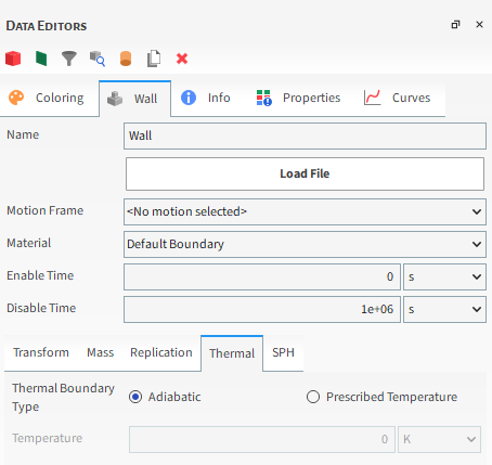
Thermal Thermal Boundary Type When Thermal Model is enabled (see also about Physics Parameters), this determines how heat conduction is calculated for the boundary. Specifically:
Adiabatic applies no heat transfer to the boundary.
Prescribed Temperature applies a constant temperature value to the boundary, as specified by the Temperature parameter.
Adiabatic; Prescribed Temperature
SPH Boundary Condition Type Select the type of SPH Boundary Condition for the imported geometry. There are three options: Free Slip, No Slip Laminar and No Slip Turbulent.
No limit Modules
(Varies)
These settings are specific to only certain external Modules and are therefore not documented in the FreeFlow User Manual. Refer to the Module's documentation (if provided) for more information.
(Varies)
See Also:
EDIT THE PARAMETERS FOR A GEOMETRY
From the Data panel, under Geometries, select the name of the geometry that you want to edit. The parameters for that geometry are displayed in the Data Editors panel. The tab named with the type of geometry you selected (for example, "Wall", "Surface", and so on) will be active.
From the Data Editors panel, enter the information you want on the active tab, being sure to select each of the various sub-tabs or dialogs that contain parameters you want to modify.
Tip: To set the same value for a parameter across multiple similar geometries, multi-select the geometries you want in the Data panel (SHIFT + left-click for a continuous group; CTRL + left-click for discontinuous items) and then change the values you want in the Data Editor panel. Only those parameters common across all selected geometries will be editable but any changes made will populate across the selected group.
See Also:
EXPORT A GEOMETRY COMPONENT TO AN STL FILE
In cases where you need to analyze or otherwise make use of your rendered geometry component outside of FreeFlow, you may choose to export it to an .stl file. This applies to any geometry components that you have previously imported. Exporting a geometry at different times for can be useful for any further analyses you may want to do.
This export ability applies also to any User Processes created from a geometry component, which exports the shape of any (whole) geometry triangles that are selected by the User Process.
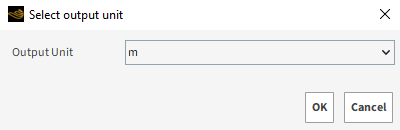
Exporting a geometry component enables you to select which units you want to use when exporting (Figure 1).
Follow the steps to export a geometry component to an STL File:
From the Data panel, under Geometries, right-click the component you want to export, point to Export, and then click Rendered Geometry.
From the Select output unit dialog, select from the Output Unit list the units you want, and then click OK.
From the Select target STL file dialog, click the drive or folder of the location to which you want to save the file.
In the File name box, enter a name for the file, and then click Save.
The steps above also apply in case you want to export an imported surface to an STL File. However, it is not possible to export surfaces created inside FreeFlow.
See Also:
From the Data panel, under Geometries, right-click the name of the geometry you want to remove, and then click Remove Geometry.
Tip: If you want to change out a geometry component for a different file, you can also choose to just replace the file. (See also Replace an Imported Geometry File.)
See Also:
REPLACE AN IMPORTED GEOMETRY FILE
Follow the steps to replace an imported geometry file:
From the Data panel, under Geometries, select the imported geometry component you want to replace.
From the Data Editors panel, select the Geometry tab and then click the Load File button.
From the Select file to import dialog, locate and select the geometry file you want to re-import, and then click Open.
From the File Import Info dialog, choose the import options you want, and then click OK
See Also:
Motion Frames are the method by which you enable geometry components (wall or surfaces) to translate, rotate, vibrate, swing, and/or move during your simulation. If a surface is attached to an Inlet/Outlet, this component will also inherit the motion assigned to the geometry. You first define your desired movement within the Motion Frame, and then assign the Motion Frame to the geometry you want to move. After setting up and applying your Motion Frames, it is a good idea to preview your motions in a Motion Preview window before processing the simulation.
What would you like to do?
See Also:
ABOUT CREATING AND APPLYING MOTION FRAMES
Creating and applying one or more Motion Frames to an imported geometry enables that component to move or animate during your simulation. You can create simple movements-including translation, rotation, vibration, and swinging motions-or more complex movements by nesting several Motion Frames, and/or by enabling six degrees of freedom (6DOF) functionality (also known as Free Body Motion).
Motion Frames work best in conjunction with the Motion Preview window as it allows you to view and test your motions before processing your simulation. (See also Preview a Motion in 3D.)
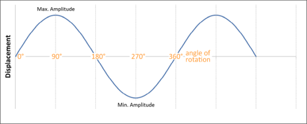
INITIAL PHASES (VIBRATION AND PENDULUM MOTIONS)
Periodic Translation (Vibration) and Periodic Rotation (Pendulum) motions are defined by specifying the amplitude and frequency values along a sine wave. The amplitude defines how far from the center point the movement translates (or rotates) and the frequency defines how many complete wave cycles will occur per second. The point along the sine wave period at which the motion begins along the sine wave is defined by the Initial Phase value. An Initial Phase value of zero degrees (default) causes the sine wave to start at the center point of the motion (Figure 1). For a simple linear vibration moving back and forth along the X axis, the frame would start at the zero position, move to the right most limit (maximum amplitude), reverse direction past the zero position to the left most limit (minimum amplitude), and then complete the cycle by reversing direction again to the zero (or 360 degree) position.
By comparison, changing the Initial Phase value to 90 degrees moves the starting point of the sine wave to the maximum amplitude, or in the simple linear vibration example, the right-most limit along the X axis (Figure 2). In this example, the frame would start its motion at the right-most limit along the X axis, then reverse direction past the zero position to the left most limit (minimum amplitude), and then reverse again to end its cycle at the right-most limit position.
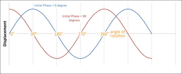
Changing the Initial Phase can be useful in cases where you want the center of the motion to remain the same but want the motion itself to begin from a non-center position. This is especially useful when combining two motions to create a complex motion.
For example, to create a circular vibration motion along the XY axes, you would create two separate vibration motions: the first along the X axis with Initial Phase at zero degrees, and the second along the Y axis with the Initial Phase at 90 degrees. This enables the vibration along the Y axis to start at its maximum (highest) position at the same time the vibration along the X axis begins its movement to the right from its center point. The combination of these two motions creates the desired circular vibration motion.
Periodic motions enable you to loop or repeat a set of motions within your simulation. When Enable Periodic Motion is turned on for a frame, the full list of motions contained within that frame will be repeated as soon as the motion with the last Stop Time completes. The amount of time between the earliest motion's Start Time and the latest motion's Stop Time is saved within FreeFlow as the periodic motion period.
This periodic motion period is useful to know when setting geometry replication as it can help you define your Replication Interval. To include an evenly spaced copy of the geometry along your periodic motion path, the Replication Interval should be equal to the periodic motion period divided by the Number of Replications you have defined.
Free body motions, including Free Body Translation and Free Body Rotations, enable the frame to move freely in response to outside forces. These forces can come from SPH elements, gravity, or from an additional force that you prescribe through the Additional Force or Additional Moment motions, the Spring-Dashpot Force or Spring-Dashpot Moment motions, or the Linear Time Variable Force or Linear Time Variable Moment motions.
Free body motions do not currently respond to other boundary interactions. So setting an object to drop freely onto another object from some height will cause the object to fall through the other object. Having that same object drop freely onto a bed of SPH elements, however, will cause the object to displace the SPH elements and slow the object's falling as expected.
An Additional Force, Spring-Dashpot Force, or Linear Time Variable Force can be added to a Free Body Translation motion in cases where you want an additional force in a given direction to affect the translation, and you want that force to be considered in the motion calculation along with the weight and gravity.
For example, to simulate a car tire rolling along a bed of SPH elements, aside from setting Free Body Translation and Free Body Rotation motions to simulate the horizontal translation and rotation of the tire, you could also add an Additional Force to account for the forward motion of the car itself. In this way, the acceleration and velocity of the translation will be affected by the SPH elements and gravity values: given the same force applied, the car moves differently when moving from dry road to a puddle of water. If only a Translation were given instead of a combined Additional Force and Free Body Translation, the velocity of the translation would remain constant no matter the conditions of the other SPH elements and forces coming into contact with it.
So too, an Additional Moment, Spring-Dashpot Moment, or Linear Time Variable Moment can be added to a Free Body Rotation motion in cases where you want an additional moment (or torque) in a given direction to affect only the rotation, and you want that additional torque to be included along with gravity in the motion calculation.
Free body motions can also have range limits applied to restrict free movement in a given direction.
Important: In order to preview a free body motion in the Motion Preview window or start processing the simulation, ensure there is a geometry component in the project that has the free body motion associated to it; otherwise, you will get an error.
In FreeFlow, you are able to add many more types of concurrent free body motions and Frames, including nested Frames, as long as free body motions of the same type (Translation or Rotation) and direction do not overlap in time.
Also, the Motion Preview window will preview the effects of gravity and any additional (prescribed) forces/moments that you define for free body motions, but will not be able to predict motions as a result of interactions with SPH elements.
Note: Free body motions are not compatible with geometry replication features.
In order to create complex motions, FreeFlow allows you to nest motion frames under other motion frames. By doing so, the nested frame (child) becomes linked to the frame above it in the tree (parent). The child motion frame will move together with the parent motion frame and will also prescribe its own motions.
Because of this, only the child frame in a nested frame situation will be assigned to a geometry, as the child inherits its parent's motions in combination with its own motions.
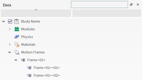
Figure 3 below shows an example of a two child frames (Frame <01> <01> and Frame <01> <02>) nested beneath a parent frame (Frame <01>).
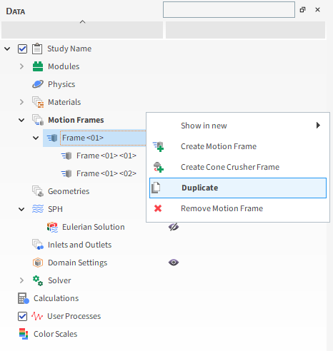
Like any other Data panel item, you can duplicate an individual Motion Frame to create an exact copy of it by right-clicking on the item and selecting the Duplicate option. This exact copy includes any nested or child Frames that exist underneath the Frame that you are copying.
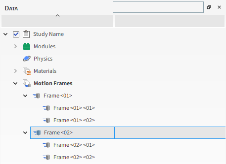
In Figure 3 below, Frame <01> <01> and Frame <01> <02> are nested or child Frames of Frame <01>. When Frame <01> is duplicated, both child Frames are duplicated as well (Figure 4), so that the new Frame <02> includes two child Frames: Frame <02> <01> and Frame <02> <02>.
MOTION FRAMES WITHIN SIMULATIONS THAT HAVE BEEN COPIED FOR RESTART PURPOSES
Motion Frames that are active at the time a processed simulation is saved for restart purposes (see also Save a Copy of a Partially Processed Simulation for Restart Purposes) will be copied to the new simulation and retain their original geometry assignments. However, even though the geometries using the frames can be removed from the copy, the copied frames themselves cannot be removed from the copy. These copied frames will also only allow changes to the Stop Time field for the existing motion (as long as the copied motion hasn't completed yet, meaning the Stop Time value is positive); new motions can be added to the existing frame, however, by clicking the Add Motion button.
In addition, only new motion frames can be assigned to new geometries in the copy; newly added geometries cannot be assigned frames copied from the original simulation, and geometries with motion frames copied from the original simulation cannot be assigned newly added motion frames.
Be aware that if you choose to use parametric expressions in either the Start Time or Stop Time fields of your original simulation project, know that only the resulting values and not the variables and/or mathematical functions you entered will be retained in the project copy you save for restart purposes.
Each Motion Frame has its own orientation reference (i.e., coordinate system) upon which its movements are based. The current (i.e., instantaneous) orientation is represented in the Motion Preview window by the axis for the Frame.
In FreeFlow, all Frames use only an implicit "local" reference, which uses the current orientation of the selected Frame to define the next movement. In this way, the reference is always moving along with the Frame.
MOTION FRAMES AND INLETS/OUTLETS
You are able to assign a Motion Frame to Inlets or Outlets. To do that you need to add a Motion Frame to the surface that is attached to that Inlet or Outlet (see also About Adding and Editing Inlets and Outlets).
See also Apply a Motion Frame to a Geometry.
MOTION FRAMES AND USER PROCESSES
User processes created for post-processing, such as cubes and cylinders, can now use motion frames to move around the domain and extract data while following geometries or SPH elements.
See also Apply a Motion Frame to a User Process.
See the images and tables below to understand how to create and apply Motion Frames to your imported Geometries.
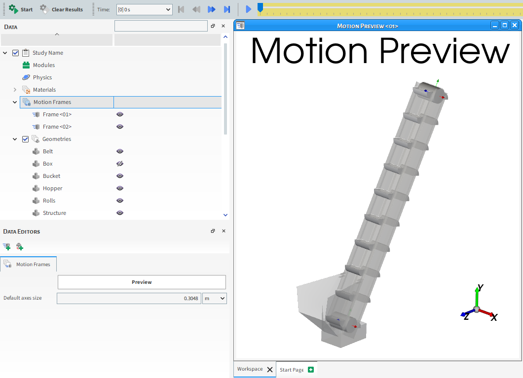
Table 1: Motion Frames parameters (Main Entity)
|
Setting |
Description |
Range |
|---|---|---|
|
Default axes size |
Sets the size of the axes used to represent the Motion Frames in the Motion Preview window. Changing the size is useful in cases where the geometries are significantly bigger or smaller than the motion axes, as seeing the axes in relation to the movement of the geometry is critical to understanding and verifying the movement setup. Affects all Motion Frames axes in the project. (See also Preview a Motion in 3D.) Note: The axes for Motion Frames are different than the axes for the windows themselves; the latter have their own display settings that you can modify. (See also About Using the Window Editors Panel to Change the Window Axes Displays.) |
Positive value |
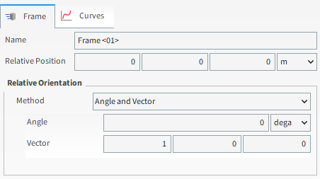
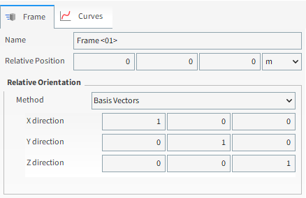
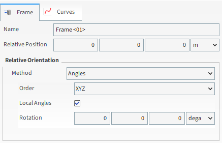
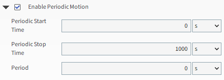
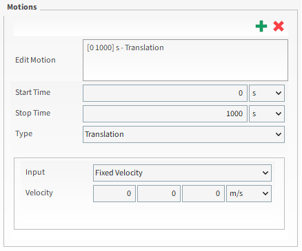
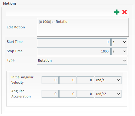
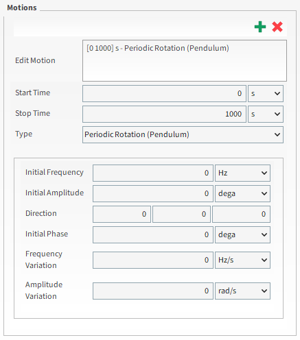
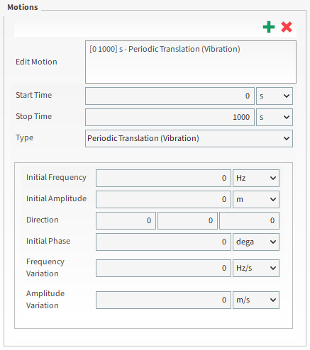
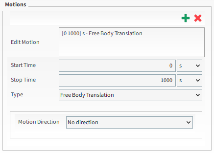
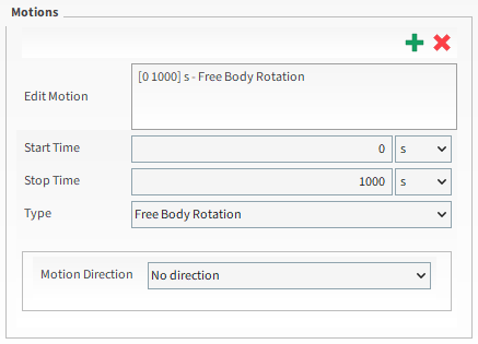
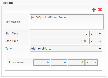
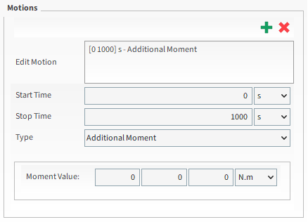
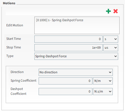
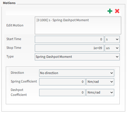
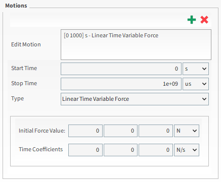
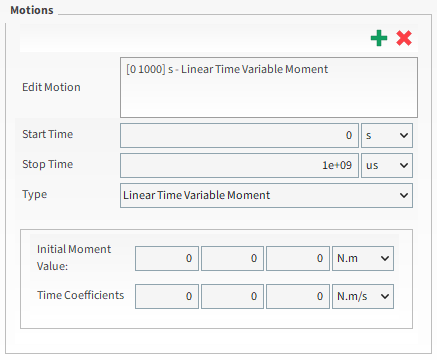

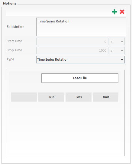
Table 2: Motion Frames parameters (Individual Frames)
|
Setting |
Description |
Range |
|---|---|---|
|
Name |
Enables you to set a unique identifier for the selected motion frame. |
99 character limit |
|
Relative Orientation |
Enables you to select how you want to define the orientation of the motion frame shape. Specifically:
|
Angles; Angle and Vector; Basis Vectors. Angle and Vector; Basis Vectors. |
|
Relative Orientation Angle and Vector | ||
|
Angle |
When Angle and Vector is selected for Orientation, this is the angle the motion frame will rotate around the Vector defined. |
Any value |
|
Vector |
When Angle and Vector is selected for Orientation, this is the X, Y, and Z components that define the vector around which the motion frame will rotate, using the Angle defined. |
No limit but the values entered will be normalized |
|
Relative Orientation Basis Vector | ||
|
X direction |
When Basis Vectors is selected for Orientation, this is the coordinate values defining the first of three directional vectors that together define the final orientation of the motion frame. Note: To ensure correct results, make sure you define this vector as orthogonal (perpendicular) to the other two vectors. |
No limit but,the values entered will be normalized |
|
Y direction |
When Basis Vectors is selected for Orientation, this is the coordinate values defining the second of three directional vectors that together define the final orientation of the motion frame. Note: To ensure correct results, make sure you define this vector as orthogonal (perpendicular) to the other two vectors. |
No limit but,the values entered will be normalized |
|
Z direction |
When Basis Vectors is selected for Orientation, this is the coordinate values defining the third of three directional vectors that together define the final orientation of the motion frame. Note: To ensure correct results, make sure you define this vector as orthogonal (perpendicular) to the other two vectors. |
No limit but,the values entered will be normalized |
|
Relative Orientation Angles | ||
|
Order |
When Angles is selected for Orientation, this defines the order in which the three Rotation text fields will be applied. |
XYZ; ZXY; YXZ; YZX; ZXY; ZYX. |
|
Local Angles |
When Angles is selected for Orientation, this defines what coordinate system will be used as a basis for the angle specified. Specifically:
|
Turns on or off |
|
Rotation |
When Angles is selected for Orientation, this is the degree of cube rotation in each of the three directions specified by the Order provided. |
Any value |
|
Keep in Place |
Specifies whether or not the motion frame to which the frame is assigned will appear to move physically from one location to another. Specifically:
Notes:
|
Turns on or off |
|
Enable Periodic Motion |
Enables the motion(s) defined for the selected frame to be repeated or looped for a defined period within the simulation. (See also Use Motion Frames to Enable Geometry Motions to be Repeated.) |
Turns on or off |
|
Periodic Start Time |
When Enable Periodic Motion is selected, this defines the amount of delay after the motion(s) Start Time and Stop Time to begin and end the motion to be repeated. Specifically:
|
Positive values |
|
Periodic Stop Time |
When Enable Periodic Motion is selected, this defines the time during the simulation when the motion(s) will stop, regardless of what is set for Stop Time. Specifically:
Tip: To ensure that the periodic motion continues for the entire simulation, keep this value set to the default (1000 s) or set it higher than your simulation duration. |
Positive values |
|
Period |
When Enable Periodic Motion is selected, this defines how much of the original motion(s) will be repeated. Specifically:
|
Positive values |
|
Edit Motion |
Lists the individual motions you have defined for the selected motion frame. Motions are automatically named in accordance with the following method: [StartTime StopTime] - Type |
Automatically determined |
|
Start Time |
The time you want the selected motion to begin.
Note: If you choose to use parametric expressions in this field, know that only the resulting value and not the variables and/or mathematical functions you enter will be retained in any project copies you save for restart purposes.
|
Positive values Tip: Tip: Check the Status panel to ensure that any variables or mathematical functions you might use results in valid values. (See also Double-Click the Status Panel to Jump to the Appropriate UI Location.) |
|
Stop Time |
The time you want the selected motion to end. Note: Any gaps of time between multiple motions will be interpreted as no movement; If you choose to use parametric expressions in this field, know that only the resulting value and not the variables and/or mathematical functions you enter will be retained in any project copies you save for restart purposes. |
Positive values Tip: Check the Status panel to ensure that any variables or mathematical functions you might use results in valid values. (See also Double-Click the Status Panel to Jump to the Appropriate UI Location.) |
|
Type |
Defines the type of movement. Specifically:
|
Translation; Rotation; Periodic Rotation (Pendulum); Periodic Translation (Vibration); Free Body Translation; Free Body Rotation; Additional Force; Additional Moment; Spring-Dashpot Force; Spring-Dashpot Moment; Linear Time Variable Force; Linear Time Variable Moment |
|
Translation Parameters | ||
|
Input |
Determines what velocity and acceleration values you want the motion to consider. Specifically:
|
Fixed Velocity; Initial and Final Velocity; Initial Velocity and Acceleration |
|
Velocity |
When Fixed Velocity is chosen for Input , this enables you to set a single translational velocity in the X, Y, and Z directions respectively. |
Any value |
|
Initial Velocity |
When Initial and Final Velocity or Initial Velocity and Acceleration is chosen for Input, this sets the starting translational velocity of the selected motion as defined in the X, Y, and Z directions respectively. A positive or negative value will prescribe the orientation of the movement over a given direction. |
Any value |
|
Final Velocity |
When Initial and Final Velocity is chosen for Input, this sets the ending translational velocity of the selected motion as defined in the X, Y, and Z directions respectively. A positive or negative value will prescribe the orientation of the movement over a given direction. |
Any value |
|
Acceleration (computed) |
When Initial and Final Velocity is chosen for Input, this displays the amount of acceleration in the X, Y, and Z directions respectively that FreeFlow calculates is required to achieve the Final Velocity given the Initial Velocity value. |
Display only; values are calculated by FreeFlow |
|
Acceleration |
When Initial Velocity and Acceleration is chosen for Input, this sets the amount of acceleration of the selected motion as defined in the X, Y, and Z directions respectively. |
Any value |
|
Final Velocity (computed) |
When Initial Velocity and Acceleration is chosen for Input, this displays the final velocity in the X, Y, Z directions respectively that FreeFlow calculates given both the Initial Velocity and Acceleration values. |
Display only; values are calculated by FreeFlow |
|
Rotation Parameters | ||
|
Initial Angular Velocity |
Sets the starting rotational (angular) velocity of the selected motion as defined in the X, Y, and Z directions respectively.
|
Any value |
|
Angular Acceleration |
Sets the amount of rotational (angular) acceleration of the selected motion as defined in the X, Y, and Z directions respectively. |
Any value |
|
Pendulum and Vibration Parameters | ||
|
Initial Frequency |
When Pendulum or Vibration is chosen for Type, this sets the starting frequency of the of the selected motion. |
Any value |
|
Initial Amplitude |
When Pendulum or Vibration is chosen for Type, this sets the starting amplitude of the selected motion. |
Any value |
|
Direction |
When Pendulum or Vibration is chosen for Type, this is the X, Y, and Z vector components that define the direction of the selected motion. Specifically:
|
No limit but values entered will be normalized |
|
Initial Phase |
When Pendulum or Vibration is chosen for Type, this determines the angular degree at which the motion begins along the sine wave that defines the oscillating movement. Specifically:
|
Any value |
|
Frequency Variation |
When Pendulum or Vibration is chosen for Type, this determines the amount of variation in frequency per unit of time for the selected motion starting from the Initial Frequency value. |
Any value |
|
Amplitude Variation |
When Pendulum or Vibration is chosen for Type, this determines the amount of variation in amplitude per unit of time for the selected motion starting from the Initial Amplitude value. |
Any value |
|
Free Body Translation and Free Body Rotation Parameters (Otherwise known as Six Degrees of Freedom (6DOF)) | ||
|
Free Motion Direction |
When Free Body Translation or Free Body Rotation are chosen for Type, this determines the axis or axes that free motion is allowed. Specifically:
|
No direction; X direction; Y direction; Z direction; X and Y directions; X and Z directions; Y and Z directions; All directions |
|
Free Body Limits | ||
|
Free Body Linear Limits |
When Free Body Translation is selected from the Type list, this enables you to limit the linear movement to occur only between the Minimum and Maximum coordinate locations you set. |
Turns on or off |
|
Free Body Angular Limits |
When Free Body Rotation is selected from the Type list, this enables you to limit the angular movement to occur only between the Minimum and Maximum coordinate locations you set. |
Turns on or off |
|
Minimum |
When Free Body Linear Limits or Free Body Angular Limits are enabled, this sets the location of the minimum limit through which you want free body movements allowed, as defined in the X, Y, and Z directions respectively. |
Any value |
|
Maximum |
When Free Body Linear Limits or Free Body Angular Limits are enabled, this sets the location of the maximum limit through which you want free body movements allowed, as defined in the X, Y, and Z directions respectively. |
Any value |
|
Additional Force and Additional Moment Parameters | ||
|
Force Value |
When Additional Force is chosen for Type , this enables you to set the amount of additional, applied force you want acted upon the selected frame. This value is defined in the X, Y, and Z axes respectively, and is itself affected by the interaction with SPH elements and gravity. Note: This motion is designed to only be used in tandem with a Free Body Translation motion. |
Any value |
|
Moment Value |
When Additional Moment is chosen for Type , this enables you to set the amount of additional, applied moment (torque) you want acted upon the selected frame. This value is defined in the X, Y, and Z axes respectively, and is itself affected by the interaction with SPH elements and gravity. Note: This motion is designed to only be used in tandem with a Free Body Rotation motion. |
Any value |
|
Spring-Dashpot Force and Spring-Dashpot Moment Parameters | ||
|
Spring Coefficient |
Defines the stiffness of the spring that attaches the frame to its original position. Note: This motion is designed to only be used in tandem with a Free Body Translation or Free Body Rotation motion. |
Any value |
|
Dashpot Coefficient |
This value when multiplied by the frame's translational or angular velocity, gives you the actual resistance force or moment. Note: This motion is designed to only be used in tandem with a Free Body Translation or Free Body Rotation motion. |
Any value |
|
Linear Time Variable Force and Linear Time Variable Moment Parameters | ||
|
Initial Force Value |
When Linear Time Variable Force is chosen for Type, this defines the initial value of the force when the motion begins at its Start Time. (See Type definitions above for full equations.) and gravity. Note: This motion is designed to only be used in tandem with a Free Body Translation motion. |
Any value |
|
Initial Moment Value |
When Linear Time Variable Moment is chosen for Type, this defines the initial value of the moment (torque) when the motion begins at its Start Time. (See Type definitions above for full equations.) Note: This motion is designed to only be used in tandem with a Free Body Rotation motion. |
Any value |
|
Time Coefficients |
When either Linear Time Variable Force or Linear Time Variable Moment are selected as Type, this coefficient is used to define the actual force (or moment) that will be applied to the motion frame by multiplying it by the motion time to obtain the load as a function of time, which will then be added to the Initial Force Value (or Initial Moment Value) defined. (See Type definitions above for full equations.) Note: This motion is designed to only be used in tandem with a Free Body Translation or Free Body Rotation motion. |
Any value |
| External Velocity Profile | ||
|
Time Series Translation |
When Time Series Translation is chosen for Type, this defines the movement displayed in the maximum, minimum, and unit (m/s) for the columns:
|
Positive Values |
|
Time Series Rotation |
When Time Series Rotation is chosen for Type, this defines the movement displayed in the maximum, minimum, and unit (m/s) for the columns:
|
Positive Values |


What would you like to do?
From the Data panel, select Motion Frames.
From the Data Editors panel, ensure Default axes size is set the way you want, and then do one of the following:
To create a new parent Motion Frame, click the Create Motion Frame button. A new Frame entry appears under Motion Frames in the Data panel.
To create a new nested (child) Motion Frame, from the Data panel, select the parent Frame entry to which you want to add a child Motion Frame, and then from the Data Editors panel, click the Create Motion Frame button. A new Frame entry appears under the parent Frame you selected in the Data panel.
From the Data panel, select the Frame you just added and then from the Data Editors panel, do all of the following:
Enter the Name, Relative Position, Relative Rotation Vector, Rotation Angle, Keep in Place, and Periodic Motion values you want. (See also About Creating and Applying Motion Frames.)
Under Motions, click the Add Motion button, and enter the motion values you want. (See also Using Motion Frames to Create Specific Movements)
Repeat step 3b for every motion you want included within the new Motion Frame.
Tip:
After creating a new Motion Frame, you must still apply the Motion Frame to an imported geometry or Custom Input to have the component itself move. (See also Apply a Motion Frame to an Imported Geometry.)
After you have applied the Motion Frame to a geometry or Custom Input, you can use the Motion Preview window to see and test the movement in 3D. (See also Preview a Motion in 3D.)
See Also:
APPLY A MOTION FRAME TO A GEOMETRY
You can add Motion Frame to any geometry, wall or surface, created or imported into FreeFlow. An useful application is to add a Motion Frame to a surface that is attached to an Inlet or Outlet (See also About Adding and Editing Inlets and Outlets.) which allows for this inlet/outlet to be moved according to the Motion Frame. To apply a Motion Frame to a geometry do all of the following:
Ensure the Motion Frame you want to apply has been created. (See also Create a Motion Frame.)
From the Data panel, select the geometry to which you want to apply a Motion Frame.
From the Data Editors panel, select the Wall/Surface tab, and then from the Motion Frame list, select the Motion Frame you want.
Tips:
Use the Motion Preview window to see and test the movement in 3D. (See also Preview a Motion in 3D.)
To apply more than one movement to a single geometry, add multiple motions to a single Motion Frame, or create a nested (child) Motion Frame and then apply the child frame to the geometry. (See also Create a Motion Frame.)
See Also:
APPLY A MOTION FRAME TO A USER PROCESS
User processes created for post-processing, such as cubes and cylinders, can now use motion frames to move around the domain and extract data while following geometries or SPH elements.
Ensure the Motion Frame you want to apply has been created. (See also Create a Motion Frame.)
From the Data panel, select the User Process to which you want to apply a Motion Frame.
From the Data Editors panel, select the Cube/Cilinder tab, and then from the Motion Frame list, select the Motion Frame you want.
Tip: To apply more than one movement to a single User Process, add multiple motions to a single Motion Frame, or create a nested (child) Motion Frame and then apply the child frame to the User Process. (See also Create a Motion Frame.)
See Also:
CREATE AND MODIFY A MOTION PREVIEW WINDOW
A Motion Preview Window is where you preview your motions to see how they affect the geometries in your simulation. Previewing is typically done after you have assigned the motion frame to the geometry but before you process the simulation.
Like other types of FreeFlow windows, you are able to define how the objects within the window and the window itself appears and function on screen. After you set up your Motion Preview window, you can choose to reuse the zoom, rotation, and pan settings in another window by saving and applying a Custom Camera Preset. You can also use the Motion Preview window as a basis for creating an animation of your motions.
What do you want to do?
See Also:
After you have defined one or more Motion Frames and have assigned them to your geometry components, a Motion Preview window is where you preview the geometry motions that you have defined. Previewing these motions before you process your simulation can allow you to catch and modify errors in your Motion Frame setup before calculations are introduced.
Notes:
The Motion Preview window will preview the effects of gravity and any additional (prescribed) forces/moments that you have defined for free body motions, but will not be able to predict motions as a result of interactions with SPH elements.
Every Motion Frame with a free body motion defined must first be associated with a geometry component in order to preview it without error on the Motion Preview window.
After you set up your Motion Frames and apply them to the components you want to move (see also About Creating and Applying Motion Frames), you use the yellow-highlighted Time Toolbar to "play" the preview (Figure: Components of a Motion Preview Window).
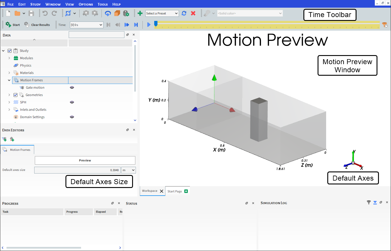
The length of the preview allowed by the Time Toolbar is based upon the Simulation Duration value you set in the Solver | Time tab (see also About Solver Parameters) with an upper limit of no more than 30,000 time steps.
Within the Motion Preview window, each Motion Frame will be represented by its own set of axes. This axes set is tied to the local or parent coordinate of the frame and should not be confused with the set of window axes, which represents only the current orientation of the window itself. (See also About Using the Window Editors Panel to Change the Window Axes Displays.)
Tip: You can change the size of the Motion Frame axes through the Default Axes Size parameter. This is located on the Motion Frames tab of the main Motion Frames entity. (See also the Table 1: Motion Frames parameters (main entity) section in the About Creating and Applying Motion Frames topic.)
As with other windows in FreeFlow, there are various ways you can change what appears in a Motion Preview window, including fonts, overlays, background colors, and grid lines. If you want to share your motions outside of FreeFlow, you can also use the Motion Preview window as a basis for creating animations.
After a simulation is processed, Motion Preview windows are still viewable but not as useful for post processing as a 3D View window. This is because after a simulation is processed, both a 3D View and a Motion Preview window will show geometry movements, but only the 3D View window will also show Sph elements.
What do you want to do?
Note:
The Motion Preview window will preview the effects of gravity and any additional (prescribed) forces/moments that you define for free body motions, but will not be able to predict motions as a result of interactions with SPH elements.
Every Motion Frame with a free body motion defined must first be associated with a geometry component in order to preview it without error on the Motion Preview window.
Ensure that the motion you want to preview has been defined in a Motion Frame. (See also Create a Motion Frame).
Ensure that the geometry or Custom Input you want to move has been assigned the Motion Frame you want. (See also Apply a Motion Frame to an Imported Geometry.)
Tip: Although you can preview a motion without first assigning it to a component, for geometries especially, it helps to see the movement if the Motion Frame is assigned to a geometry before previewing.
From the Data panel, select Motion Frames, and then from the Data Editors panel, click Preview. A new Motion Preview window appears in the Workspace.
Use the buttons on the Time toolbar (see also About the Time Toolbar) to play a preview of the motion as it might appear during the simulation.
Tip: The time step slider turns yellow to indicate when it is being used to preview motion. If the time step slider is not yellow, it is being used to show simulated time steps as usual.
Note: In preview mode, the time step slider is limited by the Simulation Duration value you set in the Solver | Time tab (see also About Solver Parameters) with an upper limit of no more than 30,000 time steps.
Tip:
Zoom, pan, tilt, and fit the image just as you would in a 3D View window by using your mouse, keyboard, an/or the Camera Visualization toolbar.
Show/hide the individual Motion Frames you want previewed by using eye icons on the Data panel.
Change attributes of the geometries and motion objects shown within the window by using the Coloring tab.
Change the attributes of the window itself, such as background colors, by using the Windows Editors panel.
For motions involving high frequency vibrations, ensure that you have set the Simulation Output Frequency (on the Solver | Time tab) low enough to properly preview the motion. (See also About Solver Parameters.)
See Also:
CHANGE A MOTION PREVIEW WINDOW
There are several ways you can change what you see in the Motion Preview window once you have created it, as explained below.
Zoom, pan, tilt, and fit the image by using your mouse, keyboard, and/or the Camera Visualization toolbar.
Change the colors and data attributes of the image, including the faces, edges, nodes, or vectors being displayed by using the Coloring tab on the Data Editors panel.
Show/hide the simulation entity you want displayed by using eye icons on the Data panel.
Change the attributes of the window itself, such as background colors, grid lines, and legend and caption details; and display options for the window axes by using the Window Editors panel.
You can also remove, rename, and show/hide a Motion Preview window just like any other window in FreeFlow.
What would you like to do?
USING THE WINDOW EDITORS PANEL TO CHANGE A MOTION PREVIEW WINDOW
From the Window Editors panel, you can modify just the selected Motion Preview window to the change attributes including the background color, font color/sizes, and synchronize the time steps displayed when two or more view windows are open. You may also use the Window Editors panel to adjust the axes display settings for all the windows in your project.
What would you like to do?
USING THE WINDOW EDITORS PANEL TO CHANGE THE SELECTED MOTION PREVIEW WINDOW
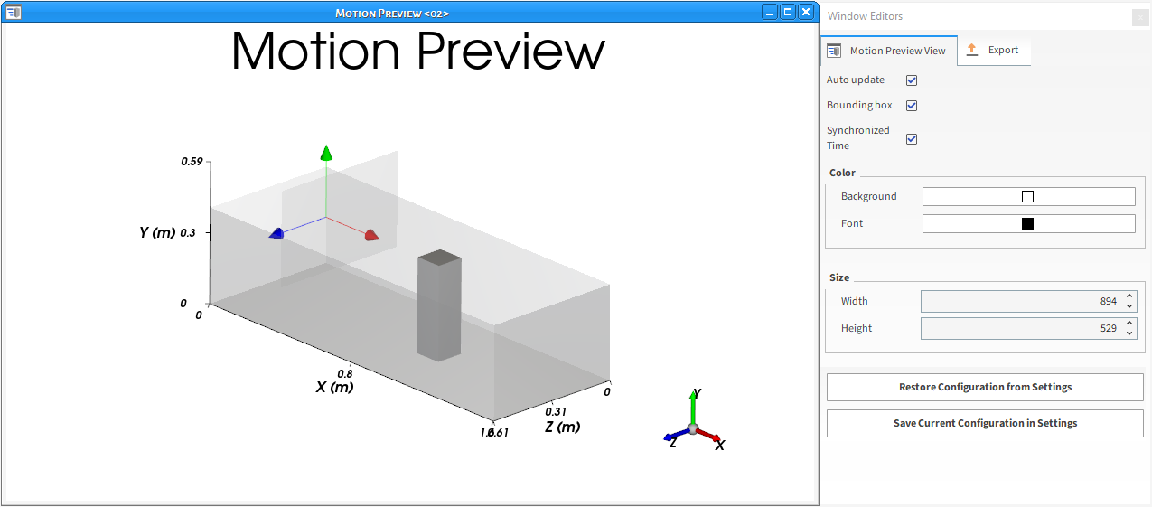
Tips:
You can also use FreeFlow Preferences to change the background color and fonts for all the Motion Preview windows in your project, instead of just the selected one. (See the "Preferences for Windows Properties" section in the About Setting Global Preferences topic.)
You can also change the window axes display for all windows in your project, including Motion Preview windows.
Note: The window axes is different from the motion frame axes, which has its own display settings. (See also About Creating and Applying Motion Frames.
In this section, we will cover only the items on the Motion Preview View tab.
You can use the Motion Preview View tab on the Window Editors panel to change how the window appears and how the data displayed within it is updated. These options include changing display items like the background color; labels, lines, and axes colors; color scale label sizes; and window height and width. In addition, you can choose to show or hide the Bounding box, which displays measurements illustrating the simulation boundaries; use Auto update to enable or prevent the view from being updated when data affecting it is changed; or choose to have multiple views updated with the same time step by using Synchronized Time.
See the image above and table below to understand more about how you can use the Window Editors panel to change a Motion Preview window.
Table 1: Motion Preview View tab options on the Window Editors panel
|
Setting |
Description |
Range |
|---|---|---|
|
Auto update |
When enabled, any change made to the display settings of the selected Motion Preview window or to the items affecting the data or settings calculated and displayed within the Motion Preview, including the time step or Geometries displayed, will be updated in the Motion Preview window automatically. Because automatically updating the window with each separate change can be computationally intensive, you can clear this option to have all calculated items and more computationally intensive display options remain unchanged in the window until you enable Auto update again. Tip: You will know when the calculations in a Motion Preview window are not being updated when you see a thick red border around the window. |
Turns on or off |
|
Bounding box |
When enabled, displays measurements illustrating the simulation boundaries in the selected Motion Preview window. |
Turns on or off |
|
Synchronized Time |
When enabled and the window (or any other window with this checkbox enabled) is selected, the details shown in this (and any other Synchronized Time) window will be updated when the current time step is changed on the Time toolbar. (See also About the Time Toolbar.) When cleared and the window is selected, only this window will be updated when the current time step is changed on the Time toolbar. Tip: To keep the time step synchronized between multiple Motion Preview or other windows, ensure each window has this option enabled. |
Turns on or off |
|
Color Background |
Enables you to change the color that appears behind the geometries in the Motion Preview window. |
Options limited by the choices in the Select Color dialog |
|
Color Font |
Enables you to change the color of the labels, borders, and axes lines displayed in the Motion Preview window. |
Options limited by the choices in the Select Color dialog |
|
Size Width |
Enables you to numerically change how wide the selected window is. Useful in cases where you need exact dimensions for image consistency, or when generating animations. |
Whole positive values between 123 and 5000. |
|
Size Height |
Enables you to numerically change how tall the window is. Useful in cases where you need exact dimensions for image consistency, or when generating animations. |
Whole positive values between 0 (zero) and 5000. |
|
Restore Configuration from Settings |
Clicking this button replaces the values set on the tab with the ones that have been saved to the (internal) FreeFlow Settings folder. |
(Button selection) |
|
Save Current Configuration in Settings |
Clicking this button overwrites the values that have been saved to the (internal) FreeFlow Settings folder with the ones currently set on the tab. |
(Button selection) |
What would you like to do?
See Also:
CHANGE WINDOW DISPLAY AND DATA UPDATE OPTIONS FOR THE SELECTED MOTION PREVIEW WINDOW
Tips:
You can also open the Window Editors panel for a window by right-clicking an empty space within the Motion Preview window (for example, the background behind the geometries), and then clicking Settings.
You can also use FreeFlow Preferences to change the background color and fonts for all the Motion Preview windows in your project, not just selected one.
To reuse in future projects the settings you made to this tab, click the Save Current Configuration in Settings button.
To apply settings you have already saved (either by previously using the Save Current Configuration in Settings button or by saving selections within the Preferences dialog) to this tab, click the Restore Configuration from Settings button.
See Also:
USING THE COLORING TAB TO CHANGE A MOTION PREVIEW WINDOW
The Coloring tab, which is located on the Data Editors panel for all simulation entities and User Processes, enables you to change the image of the items being displayed within your Motion Preview window. These include the geometry components and any user processes created from those geometry components. It also includes individual Motion Frames whose Coloring tab shows options related to the axes of the Frame that is selected in the Data panel.
Using the options on the Coloring tab is one way you can change the appearance of the items being displayed in a Motion Preview window. Visualization options for the Faces, Edges, and Nodes can be modified with the Coloring tab for any of the following entities:
Inlets
User Process created from any of the above entities
In addition, when an individual Motion Frame is selected in the Data panel, the Coloring tab for that entity shows options related to the axes of the selected Frame (Figure 1).
PARAMETERS DEFINITIONS
See the images and tables below to help you understand how to use the Coloring tab to change a view for selected entity.
Figure 3.51: Coloring tab when a Motion Frame is selected in the Data panel and a Motion Preview window is selected
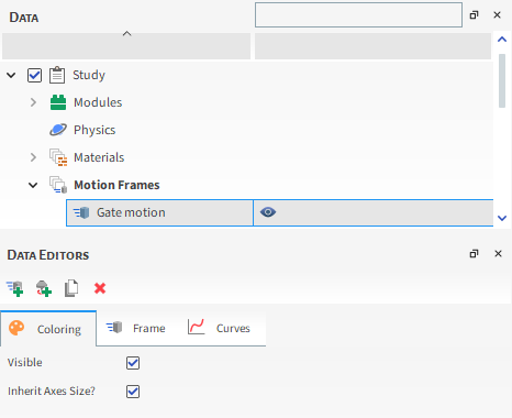
Table 1: Coloring tab parameter options for a Motion Frame when a Motion Preview window is selected
|
Setting |
Description |
Range |
|---|---|---|
|
Visible |
When enabled, shows the selected entity in the active view window. Note: This is the same as using the Data panel eye icon. |
Turns on or off |
|
Inherit Axes Size? |
When enabled, allows the selected Frame to use the same axes size as what was set in the main Motion Frames entity (see also About Creating and Applying Motion Frames to Imported Geometries). When cleared, enables you to set a unique axes size for the selected Motion Frame. |
Turns on or off |
|
Axes Size |
When the Inherit Axes Size? checkbox is cleared, this defines the custom axes size for the selected Frame. |
Positive value |
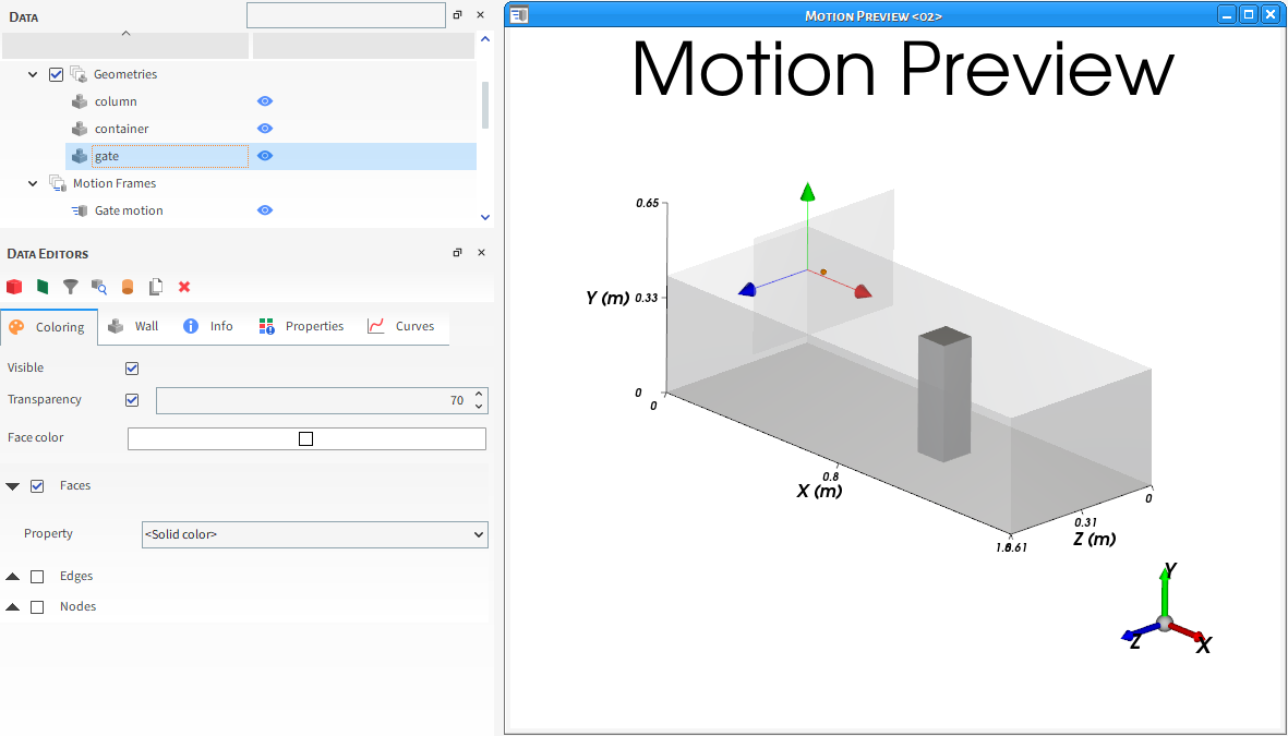
Table 2: Coloring tab parameter options for a geometry component when a Motion Preview window is selected
|
Setting |
Description |
Range |
|---|---|---|
|
Visible |
When enabled, shows the selected entity in the active view window. Note: This is the same as using the Data panel eye icon. |
Turns on or off |
|
Transparency |
Enables boundaries to be drawn transparently in the selected view window. A value of 0 (zero) makes the faces completely solid or opaque. A value of 100 makes the faces completely transparent or hidden. |
Turns on or off; 0-100 |
|
Color |
When Faces, Edges, and/or Nodes are selected and the Property is <Solid Color>, this enables the selected display type to be colored in the one solid color chosen. Note: For Faces, Transparency options affect how opaque this color appears in the view. |
Options limited by the Select Color dialog |
|
Faces |
Enables the entire surface of the entity to be visible and affected by the various Faces coloring options. |
Turns on or off |
|
Property |
Three separate lists under Faces, Edges, and Nodes respectively provide properties and other color options that apply to the display type within which the list is contained. Specifically:
|
<Solid color>; List of properties automatically generated from the Properties tab |
|
Show on Node? |
When Faces is enabled and a property is selected from the Property list under Faces, this enables the visualization of the selected property to be evenly interpolated across the entity for a smoother visualization. |
Turns on or off |
|
Edges |
Enables only the edges bordering the components making up the entity boundaries visible and affected by the various Edges coloring options. |
Turns on or off |
|
Width |
When Edges is selected, this changes the thickness of the lines used to draw the borders. Entering 1 will provide the narrowest line. |
Positive values |
|
Nodes |
Enables the points marking the intersections of the entity's individual components to be visualized as dots and affected by the various Nodes coloring options. |
Turns on or off |
|
Point Size |
When Nodes is selected, this changes the size of the dots used to draw the nodes. Entering 1 will provide the smallest dot. |
Positive values |
What would you like to do?
See Also:
USE THE COLORING TAB TO CHANGE THE MOTION PREVIEW FOR A FRAME
From the Workspace, select the Motion Preview window to which you want to apply changes. (See also Preview a Motion in 3D.)
From the Data panel, do one of the following:
Under Geometries, select the geometry component or inlet that you want to change.
Under Motion Frame, select the Frame you want to change.
From the Data Editors panel, select the Coloring tab, and then change the settings that you want. The changes you make are shown automatically in the Motion Preview window.
See Also:
USE MOTION FRAMES TO CREATE SPECIFIC MOVEMENTS
Once you know how to create and apply Motion Frames to an imported geometry (see also About Creating and Applying Motion Frames to Imported Geometries), there are many different types of movements you can create. Use this section to learn more about how to create some specific movements for your geometries.
What would you like to do?
Use Motion Frames to Enable a Regularly Swinging Boundary (for example, a Pendulum)
Use Motion Frames to Enable a Geometry to Freely Move Linearly
Use Motion Frames to Enable a Geometry to Freely Move Linearly with an Added Force
Use Motion Frames to Enable a Geometry to Freely Rotate Around its Center Point
Use Motion Frames to Enable Multiple Movements of a Geometry in one Simulation
USE MOTION FRAMES TO ENABLE A GEOMETRY TO MOVE LINEARLY
Ensure the geometry you want to move has already been imported.
Create a Motion Frame as you normally would (see also Create a Motion Frame), but under Motions (step 3b), ensure that you do all of the following:
Determine when you want the motion to start and stop by entering the values you want for Start Time and Stop Time.
From the Type list, select Translation.
From the Input list, do one of the following:
To set only a fixed velocity with no acceleration, select Fixed Velocity, and then enter the Velocity you want in the X, Y, and Z axes respectively.
To set both the initial and final velocity and have FreeFlow compute the acceleration required to achieve those values, select Initial and Final Velocity and then enter the Initial Velocity and Final Velocity you want in the X, Y, and Z axes respectively.
To set both the initial velocity and the acceleration values and then have FreeFlow compute the final velocity that results from those values, select Initial Velocity and Acceleration and then enter the Initial Velocity and Acceleration values you want in the X, Y, and Z axes respectively.
Apply the new Motion Frame to the geometry you want to move. (See also Apply a Motion Frame to an Imported Geometry.)
Use the Motion Preview window to see and test the movement in 3D. (See also Preview a Motion in 3D.)
See Also:
USE MOTION FRAMES TO ENABLE A GEOMETRY TO ROTATE AROUND ITS CENTER POINT
Ensure the geometry you want to move has already been imported.
Create a Motion Frame as you normally would (see also Create a Motion Frame), but ensure that you do all of the following:
For Relative Position, enter the location of the geometry's center point.
Under Motions (step 3b), do all of the following:
Determine when you want the motion to start and stop by entering the values you want for Start Time and Stop Time.
From the Type list, select Rotation.
Enter the Initial Angular Velocity you want in the X, Y, and Z axes respectively.
If you want velocity affected by acceleration, enter the Angular Acceleration you want in the X, Y, and Z axes respectively.
Apply the new Motion Frame to the geometry you want to move. (See also Apply a Motion Frame to an Imported Geometry.)
Use the Motion Preview window to see and test the movement in 3D. (See also Preview a Motion in 3D.)
See Also:
USE MOTION FRAMES TO ENABLE A REGULARLY SWINGING BOUNDARY (E.G. A PENDULUM)
Note: Use this procedure when the swinging motion is applied to the geometry in a predictable and regular manner. To enable a boundary that swings freely based upon SPH elements acting upon it, see the procedure Use Motion Frames to Enable a Geometry to Rotate Freely Around a Non-Center Point (for example, a Gate or Rubber Curtain).
Ensure the geometry you want to move has already been imported.
Create a Motion Frame as you normally would (see also Create a Motion Frame), but under Motions (step 3b), ensure that you do all of the following:
Determine when you want the motion to start and stop by entering the values you want for Start Time and Stop Time.
From the Type list, select Periodic Rotation (Pendulum).
Enter the Initial Frequency and Initial Amplitude.
For Direction, enter the X, Y, Z vector components defining the 2D plane upon which the swinging will occur.
For Initial Phase, enter the starting angular degree (Plane Angle) you want to use.
If you want the frequency or amplitude to vary per unit of time for the selected motion, enter what you want for Frequency Variation and Amplitude Variation.
Apply the new Motion Frame to the geometry you want to move. (See also Apply a Motion Frame to an Imported Geometry.)
Use the Motion Preview window to see and test the movement in 3D. (See also Preview a Motion in 3D.)
See Also:
USE MOTION FRAMES TO ENABLE A VIBRATING BOUNDARY
Ensure the geometry you want to move has already been imported.
Create a Motion Frame as you normally would (see also Create a Motion Frame), but under Motions (step 3b), ensure that you do all of the following:
Determine when you want the motion to start and stop by entering the values you want for Start Time and Stop Time.
From the Type list, select Periodic Translation (Vibration).
Enter the Initial Frequency and Initial Amplitude.
For Direction, enter the X, Y, Z vector components defining the direction over which the vibrating motion will occur.
For Initial Phase, enter the starting angular degree (Plane Angle) you want to use.
If you want the frequency or amplitude to vary per unit of time for the selected motion, enter what you want for Frequency Variation and Amplitude Variation.
Apply the new Motion Frame to the geometry you want to move. (See also Apply a Motion Frame to an Imported Geometry.)
Use the Motion Preview window to see and test the movement in 3D. (See also Preview a Motion in 3D.) Tip:For motions involving high frequency vibrations, ensure that you have set your Solver | Time Interval low enough to properly preview the motion. (See also About Solver Parameters.)
See Also:
USE MOTION FRAMES TO ENABLE A GEOMETRY TO FREELY MOVE LINEARLY
Ensure the geometry you want to move has already been imported.
Create a Motion Frame as you normally would (see also Create a Motion Frame), but under Motions (step 3b), ensure that you do all of the following:
Determine when you want the motion to start and stop by entering the values you want for Start Time and Stop Time.
From the Type list, select Free Body Translation.
From the Free Motion Direction list, select the axis or axes that you want free motion enabled. Tip:To have Free Motion enabled in every possible direction, select All directions.
Apply the new Motion Frame to the geometry you want to move. (See also Apply a Motion Frame to an Imported Geometry.) Note: With free body motions, missing this step will result in errors when you later try to either preview the motion or process the simulation.
Use the Motion Preview window to see and test the effects of gravity. (See also Preview a Motion in 3D.)
Note: Because the movement of a geometry with Free Motion is directly affected by the interaction with SPH elements yet to be calculated, the Motion Preview window will only be able to preview the effects of gravity and any additional (prescribed) forces/moments you have defined.
See Also:
USE MOTION FRAMES TO ENABLE A GEOMETRY TO FREELY MOVE LINEARLY WITH AN ADDED FORCE
Ensure the geometry you want to move has already been imported.
Create a Motion Frame with a Free Body Translation Motion Type. (See also Use Motion Frames to Enable a Geometry to Freely Move Linearly.)
Add a second Motion to the selected Frame by clicking the Add Motion button, and then do all of the following:
Determine when you want the motion to start and stop by entering the values you want for Start Time and Stop Time.
From the Type list, select Additional Force.
For Force Value, enter the X, Y, and Z components defining the amount of additional, applied force you want acted upon the selected Frame.
Apply the new Motion Frame to the geometry you want to move.
Note: With free body motions, missing this step will result in errors when you later try to either preview the motion or process the simulation.
Use the Motion Preview window to see and test the effects of gravity and the additional (prescribed) forces/moments that you defined. (See also Preview a Motion in 3D.)
Note: Because the movement of a geometry with Free Motion is directly affected by the interaction with SPH elements yet to be calculated, the Motion Preview window will only be able to preview the effects of gravity and any additional (prescribed) forces/moments that you have defined.
See Also:
USE MOTION FRAMES TO ENABLE A GEOMETRY TO FREELY ROTATE AROUND ITS CENTER POINT
Ensure the geometry you want to move has already been imported.
Create a Motion Frame as you normally would (see also Create a Motion Frame), but ensure that you do all of the following:
For Relative Position, enter the location of the geometry's center point.
Under Motions (step 3b), do all of the following:
Determine when you want the motion to start and stop by entering the values you want for Start Time and Stop Time.
From the Type list, select Free Body Rotation.
From the Free Motion Direction list, select the axis or axes that you want free motion enabled. Tip:To have Free Motion enabled in every possible direction, select All directions.
Apply the new Motion Frame to the geometry you want to move. (See also Apply a Motion Frame to an Imported Geometry.)
Note: With free body motions, missing this step will result in errors when you later try to either preview the motion or process the simulation.
Use the Motion Preview window to see and test the effects of gravity. (See also Preview a Motion in 3D.)
Note: Because the movement of a geometry with Free Motion is directly affected by the interaction with SPH elements yet to be calculated, the Motion Preview window will only be able to preview the effects of gravity and any additional (prescribed) forces/moments you have defined.
See Also:
USE MOTION FRAMES TO ENABLE A GEOMETRY TO FREELY ROTATE AROUND A NON-CENTER POINT WITH ADDED TORQUE (E.G., A GATE OR RUBBER CURTAIN)
Ensure the geometry you want to move has already been imported.
Create a Motion Frame with a Free Body Rotation Motion Type (see also Use Motion Frames to Enable a Geometry to Freely Rotate Around its Center Point) but be sure to set the Frame Relative Position to be the coordinate location of the point you want the geometry to rotate around.
Add a second Motion to the selected Frame by clicking the Add Motion button, and then do all of the following:
Determine when you want the motion to start and stop by entering the values you want for Start Time and Stop Time.
From the Type list, select Additional Moment.
For Moment Value, enter the X, Y, and Z components defining the amount of additional, applied moment (torque) you want acted upon the selected Frame.
Apply the new Motion Frame to the geometry you want to move. (See also Apply a Motion Frame to an Imported Geometry.)
Note: With free body motions, missing this step will result in errors when you later try to either preview the motion or process the simulation.
Use the Motion Preview window to see and test the effects of gravity and the additional (prescribed) forces/moments that you defined. (See also Preview a Motion in 3D.)
Note: Because the movement of a geometry with Free Motion is directly affected by the interaction with SPH elements yet to be calculated, the Motion Preview window will only be able to preview the effects of gravity and any additional (prescribed) forces/moments that you have defined.
See Also:
USE MOTION FRAMES TO ENABLE MULTIPLE MOVEMENTS OF A GEOMETRY IN ONE SIMULATION
Ensure the geometry you want to move has already been imported.
Create a Motion Frame as you normally would (see also Create a Motion Frame).
Do one of the following:
To create an additional motion within the selected Motion Frame, click the Add Motion button, and set up the additional motion as you normally would.
To create a separate Frame linked to the selected Motion Frame, do the following:
Click the Add Motion Frame button. A nested (child) Frame appears beneath the original Frame in the Data panel.
From the Data panel, select the new Frame, and then set up the motion as you normally would.
Apply the Motion Frame to the geometry you want to move. (See also Apply a Motion Frame to an Imported Geometry.) Specifically:
For multiple motions within one Motion Frame, apply the single Motion Frame to the geometry. All motions within the Motion Frame will be applied.
For multiple nested Motion Frames, apply the lowest-level child Motion Frame to the geometry. All Motion Frames linked to the child, including their defined motions, will be applied.
Use the Motion Preview window to see and test the movement in 3D. (See also Preview a Motion in 3D.)
See Also:
USE MOTION FRAMES TO ENABLE GEOMETRY MOTIONS TO BE REPEATED
Ensure the geometry you want to have periodic motions has already been imported.
Create a Motion Frame as you normally would (see also Create a Motion Frame), but but for part 3a, do the following:
Be sure that you enable the Enable Periodic Motion check box.
In the Periodic Start Time box, enter the amount of delay after the motion(s) Start Time and Stop Time to begin and end the motion to be repeated.
In the Periodic Stop Time box, enter the exact time you want the motion(s) to stop, regardless of what is set for its Stop Time.
Tip: To ensure that the periodic motion continues for the entire simulation, keep this value set to the default (1000 s) or set it higher than your simulation duration.
In the Period box, enter how much of the original motion(s) will be repeated.
Continue setting up your Motion Frame as you normally would.
Use the Motion Preview window to see and test the movement in 3D. (See also Preview a Motion in 3D.)
Tip: To have the periodic motion appear at simulation onset, keep both the Start Time and Periodic Start Time zero (0).
See Also:
FreeFlow enables you to specify unique properties for both solid and fluid materials. Geometries and fluid elements used in your simulation can each have specific materials, allowing you to ensure that the various components being simulated interact with each other in as realistic a way as possible.
What would you like to do?
Learn more About Modifying Solid Material Compositions
See also
ABOUT MODIFYING SOLID MATERIAL COMPOSITIONS
By default, FreeFlow defines one Solid Material set for each simulation (Default Boundary). While you can modify the settings for this default Materials and also add additional Material definitions if you choose, you cannot remove them from the simulation.
Materials you define here will be used when defining the parameters for Geometries.
MATERIALS AND EXTERNAL MODULES
If you have enabled one or more external Modules that affect your Materials settings, you might also have separate, module-specific settings that you can define. Refer to the Module's documentation (if provided) for more information.
MATERIALS PARAMETER DEFINITIONS
Use the figure and table below to help you understand the various parameters you can modify for Materials.
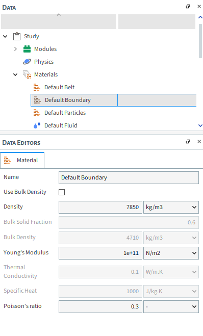
Table 1: Material parameter options (all available)
|
Setting |
Description |
Range |
|---|---|---|
|
Name |
Enables you to specify a unique identifier for the Material. |
99 character limit |
|
Use Bulk Density |
When selected, the Density of the solid materials will be calculated using both the Bulk Density and the Bulk Solids Fraction for Materials values. When cleared, the Density value you enter directly will be used instead. Note: No matter what you choose here, only the Density value - either entered directly by you or calculated by FreeFlow (and shown grayed-out) based upon the bulk density values you provided - is used for calculations with Boundaries or Belts. |
Turns on or off |
|
Density |
No matter whether this value is entered by you or is calculated by FreeFlow (and shown grayed-out) based upon the bulk density values you provided, only this value will be used for Belt or Boundary calculations. For SPH elements this is the value that will be applied as the Fluid Density. |
Positive values |
|
Bulk Solid Fraction |
For all Materials that have the Use Bulk Density check box enabled, this number is applied to the (disabled) Density value of the Material. For all Materials that have the Use Bulk Density checkbox cleared, this number is applied to the (disabled) Bulk Density of the value. Note: One minus this value is the void fraction (also known as void ratio) of the Materials. (The default void fraction is 0.4.) Void fraction or porosity is a measure of the void spaces in a material. It is a fraction of the volume of voids over the total volume, between 0 and 1, or as a percentage between 0 and 100%. |
Between 0 and 1 |
|
Bulk Density |
The bulk density or apparent density of a material is defined as the mass of particles divided by the total volume they occupy. The total volume includes particle volume, inter-particle void volume, and internal pore volume. Therefore, bulk density is not an intrinsic property of a material; it can change depending upon how the material is handled and compacted; i.e., it depends upon the Bulk Solid Fraction. |
Positive values |
|
Young's Modulus |
A measure of the capacity of a material to withstand changes in length when under lengthwise tension or compression. Defines the relationship between force per unit area and proportional deformation, and is assigned as separate values to each SPH element and boundary material defined. Applied in contact stiffness calculations used in the models for normal and tangential forces for interactions between SPH elements and Boundaries or Belts. In general, the higher the value, the more accurate the results but the longer the processing time. |
Positive values |
|
Thermal Conductivity |
When Thermal Model is enabled (see also About Physics Parameters), this sets the thermal conductivity value for the material. |
Any value |
|
Specific Heat |
When Thermal Model is enabled (see also About Physics Parameters), this sets the specific heat value for the material. |
Any value |
|
Poisson's Ratio |
This sets the Poisson's Ratio value for the material. Note: Even though you are always able to set this parameter, it will only be used in the following scenarios:
|
Any value Tip: Most materials will have a Poisson's Ratio value ranging between 0.0 and 0.5 |
See Also:
ABOUT MODIFYING FLUID MATERIAL COMPOSITIONS
By default, FreeFlow defines a Fluid Material. While you can modify the settings for this default Material and also add additional Material definitions if you choose, you cannot remove it from the simulation.
Materials you define here will be used when defining the parameters for the Fluid phase, and its interactions.
FLUID MATERIALS AND EXTERNAL MODULES
If you have enabled one or more external Modules that affect your Materials settings, you might also have separate, module-specific settings that you can define. Refer to the Module's documentation (if provided) for more information. (See also FreeFlow Simulation Entities that can be Affected by Modules.)
FLUID MATERIALS PARAMETER DEFINITIONS
Use the figures and table below to help you understand the various parameters you can modify for Fluid Materials.
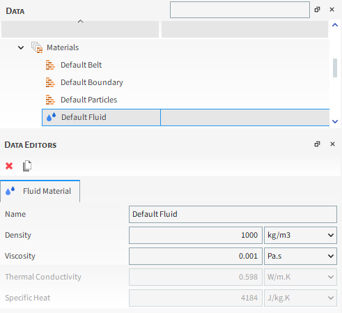
Table 1: Fluid Material Parameter Options
|
Setting |
Description |
Range |
|---|---|---|
|
Name |
Enables you to specify a unique identifier for the Material. |
99 character limit |
|
Density |
Defines the fluid material density. |
Positive values |
|
Viscosity |
Defines the fluid material dynamic viscosity. |
Positive values |
|
Thermal Conductivity |
When Thermal Model is enabled (see also About Physics Parameters), this sets the thermal conductivity value for the material. |
Any value |
|
Specific Heat |
When Thermal Model is enabled (see also About Physics Parameters), this sets the specific heat value for the material. |
Any value |
*While low sound speed can leed to numerical instabilities, high sound speeds increase the simulation cost due to the smaller time step. Refer to the SPH technical manual for guidelines on selecting the material sound speed.
See Also:
The SPH parameters available define how the simulation of fluid flow is going to be calculated.
FreeFlow uses an SPH (Smoothed-Particle Hydrodynamics) technique to perform fluid flow simulations. To ensure that the simulation is a good representation of the physics involved, you have control of several parameters that set how the SPH method is going to work in a simulation. Below you can learn more about these parameters.
To learn more about how this model is calculated, refer to the SPH Technical Manual. (From the FreeFlow Help menu, point to Manuals and then click SPH Technical Manual).
ABOUT THERMAL MODELING
FreeFlow includes an option for thermal modeling in an SPH simulation. To learn more about setting up and using SPH Thermal model in FreeFlow, refer to the Thermal Model topic under the Physics Section.
When setting up an SPH simulation, you have the option of using the Eulerian Solution feature. By default it is enabled. This option allows you to obtain interpolated results for SPH properties. This option may result in more use of computational resources. If you want to disable it, you can do so by clearing the check box Eulerian Solution under the SPH item on the data panel. To learn more about setting up and using Eulerian Solution in FreeFlow, refer to About SPH Eulerian Solution topic in Analyzing a Simulation Chapter.
SPH PARAMETERS AVAILABLE IN FreeFlow
The SPH parameters in FreeFlow can be edited from the SPH entity on the data panel. They are divided into two categories: the SPH Model Parameters with the basic setup needed to perform an SPH simulation, and an Advanced tab, with parameters that allow a fine-tuning of the simulation.
Use the figure and table below to help you understand the various SPH parameters you can set for a simulation project in the SPH Model Parameters tab, according to each Solver.
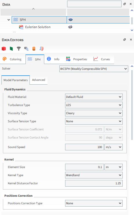
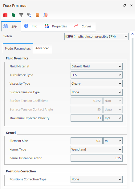
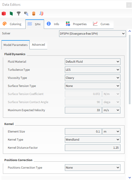
Table 1: SPH Solver Settings
|
Setting |
Description |
|---|---|
|
WCSPH (Weakly Compresible SPH) |
The Weakly Compressible SPH solver is suitable for simulating incompressible fluids, by using an artificial equation of state to compute the relation between pressure and density. |
|
IISPH (Implicit Incompressible SPH) |
The Implicit Incompressible SPH solver is also suitable for simulating incompressible fluids. In this formulation, the fluid incompressibility constraint is enforced by solving a system of linear equations at each simulation time, to compute pressure values that lead to element velocities and displacements that satisfy the constraint. This treatment allows to solve the flow equations with larger time steps than the ones needed for the Weakly Compressible SPH (WCSPH) formulation. |
| DFSPH (Divergence-free SPH) BETA |
The Divergence-free SPH solver is also suitable for simulating incompressible fluids. This solver can be considered an extension of the IISPH formulation, because both enforce a constant density value through the solution of a Poisson pressure equation. However, DFSPH introduces an additional step in which the divergence-free condition is enforced on the velocity field. Note: The DFSPH can only be used if the Experimental (Beta) Features checkbox is enabled on the Options | Preferences | Additional Features dialog. Important: Note that beta features have not been fully tested and validated. Ansys, Inc. makes no commitment to resolve defects reported against these prototype features. However, your feedback will help us improve the overall quality of the product. We will not guarantee that the projects using this beta feature will run succesfully when the feature is finally released so you may, therefore, need to modify the projects. |
Table 2: SPH Model Parameters Tab
|
Setting |
Description |
Range |
|---|---|---|
|
Fluid Dynamics | ||
|
Fluid Material |
Allows you to choose the fluid material that will be used in the simulation. (see also About Modifying Fluid Material Compositions). |
Automatically Determined |
|
Turbulence Type |
Defines the turbulence modeling approach.
For additional details about these models, see the SPH Technical Manual. (From the FreeFlow program Help menu, point to Manuals, and then click SPH Technical Manual.) |
Laminar; LES |
|
Viscosity Type |
Defines the viscosity model used in the calculation of SPH element acceleration due to viscous forces flow.
For additional details about these models, see the SPH Technical Manual. (From the FreeFlow program Help menu, point to Manuals, and then click SPH Technical Manual.) |
Cleary; Morris |
|
Surface Tension Type | Defines the surface tension model used to model free surfaces.
Note: The Pairwise Potential can only be used if the Experimental (Beta) Features checkbox is enabled on the Options | Preferences | Additional Features dialog.
If CSF or Pairwise Potential model are enabled, a new parameter will be required:
Important: When the Pairwise Surface Tension type is selected, the Surface Tension Boundary Angle and the Capillary Friction Coefficient will be available for the specified geometry, located in the Wall | SPH tab (See Imported wall, SPH parameters in the Data Editors panel). |
None; CSF; CSS; Pairwise Potential |
| Sound Speed / Maximum Expected Velocity | For WCSPH, the Sound Speed, which is about 10x the maximum expected velocity for the simulation, must be set here. For IISPH and DFSPH, the value is the Maximum Expected Velocity for the simulation. | Positive Numbers [m/s] |
|
Kernel | ||
|
Element Size |
Defines the size of an SPH element. |
Positive Values |
|
Kernel Type |
Defines the type of kernel function used for SPH calculations
For additional details about these models, see the SPH Technical Manual. (From the FreeFlow program Help menu, point to Manuals, and then click SPH Technical Manual.) |
Cubic; Quintic; Wendland |
|
Kernel Distance Factor |
Defines the kernel distance factor, which affects the size of the kernel support. |
Positive Values |
|
Positions Correction | ||
|
Positions Correction Type |
Defines the formulation applied to prevent SPH elements from clumping together and distribute them more evenly in space.
For additional details about these models, see the SPH Technical Manual. (From the FreeFlow program Help menu, point to Manuals, and then click SPH Technical Manual.) |
None; XSPH; Shift |
SPH ADAPTIVE SIZING PARAMETER DEFINITIONS
The SPH adaptive sizing parameters are shown in Figure 3.58: SPH Adaptive Sizing Parameters, the image presents the default configuration for this feature.
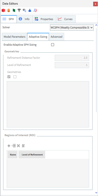
Table 3.6: SPH Adaptive Sizing Parameters Tab
| Setting | Description | Range |
|---|---|---|
|
Enable Adaptive Sizing |
A checkbox to turn on or turn off the refinement of SPH elements. The default value is off. |
On or Off |
|
Geometries | ||
|
Refinement Distance Factor |
Determines the distance from the geometry to perform the refinement process. Note: The SPH element will be refined if its distance from the boundary is lower than the product of SPH size times the Refinement Distance Factor. See SPH Adaptive Sizing for more details. |
Only integers and positive values bigger than zero. Default value is 2.5. Note: You can insert zero as value, but then, no SPH element will be refined. |
|
Level of Refinement |
Determines how much to refine the SPH element, the new SPH size will be given by
Note: A new SPH property named Refinement Count is created, see About Properties. See SPH Adaptive Sizing for more details about the refinement process. |
Only integers and positive values bigger than zero. It is recommended to use an integer value equal to 1 or 2. Default value is 1 for geometries and 0 for ROI. Note: You can insert zero as value, but then, no SPH element will be refined. |
|
Geometries (checkbox) |
Select the boundary (geometry) to use as reference to create the refinement process. |
Turn on or off the geometry as reference for the refinement process. |
|
Regions of Interest (ROI) | ||
|
Name |
Select the ROI bodies, which internal SPH elements will be refined. |
Total number of ROI bodies created in the study. |
|
Level of Refinement |
Determines how much to refine the SPH element, the new SPH size will be given by
Note: A new SPH property named Refinement Count is created, see About Properties. See SPH Adaptive Sizing for more details about the refinement process. |
Only integers and positive values bigger than zero. It is recommended to use an integer value equal to 1 or 2. Default value is 1 for geometries and 0 for ROI. Note: You can insert zero as value, but then, no SPH element will be refined. |

SPH ADVANCED PARAMETER DEFINITIONS
Use the figure and table below to help you understand the various SPH parameters you can set for a simulation project in the Advanced tab.
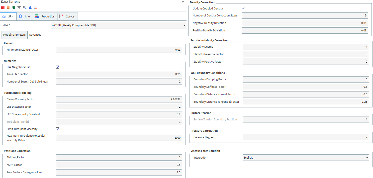
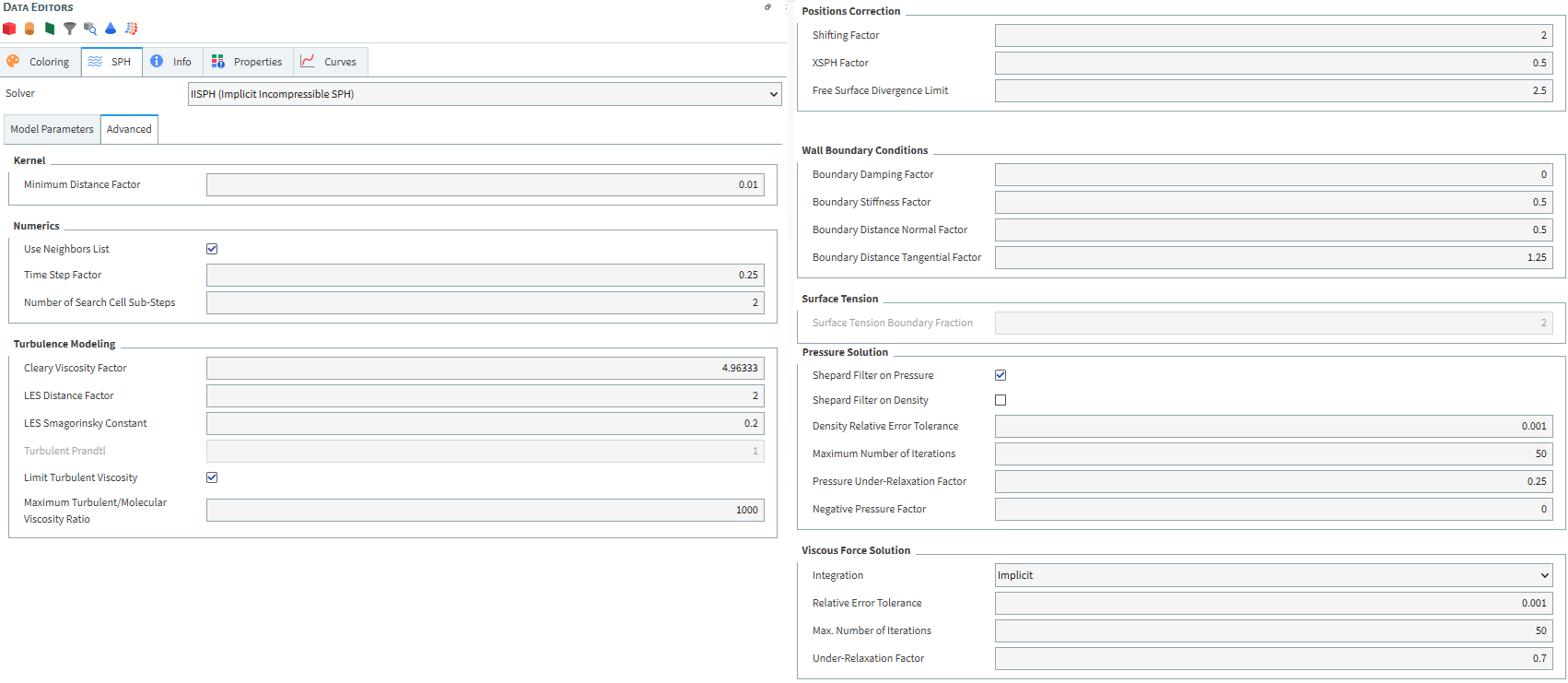
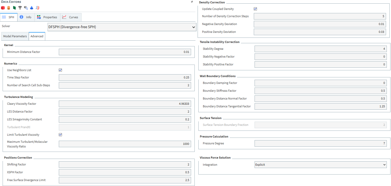
Table 3: SPH Advanced Parameters Tab
|
Setting |
Description |
Range |
|---|---|---|
|
Kernel | ||
|
Minimum Distance Factor |
Defines the factor used to calculate the minimum distance between SPH elements in order to avoid singularities. |
Positive Values |
|
Numerics | ||
|
User Neighbors List |
Allows FreeFlow to use a neighbors list which is stored in memory. This will speed up the simulation, but if the number of elements in the list exceeds the system memory available, an allocation error may occur. |
On or Off |
|
Time Step Factor |
Defines the coefficient used to compute the SPH solver time step. |
Positive Values |
|
Number of Search Cell Sub-Steps |
Defines the coefficient that is used to define the search cell size. |
Positive Values |
|
Turbulence Modelling | ||
|
Cleary Viscosity Factor |
Defines the coefficient used in the Cleary formulation of the acceleration due to viscous forces. |
Positive Values |
|
LES Distance Factor |
Defines the characteristic length used to compute the turbulent viscosity term. |
Positive Values |
|
LES Smagorinsky Constant |
Defines the Smagorinsky constant used to compute the turbulent viscosity term. |
Positive Values |
| Turbulent Prandtl | Available when Thermal Model is enabled. Defines the Prandtl Number used in the SPH HTC Calculator module for turbulent flows. |
Positive Values |
|
Positions Correction | ||
|
Shifting Factor |
Defines the shifting factor for the Shift approach. |
Positive Values |
|
XSPH Factor |
Defines the XSPH factor used for the XSPH position correction model. |
Positive Values |
|
Free Surface Divergence Limit |
Defines the concentration gradient reference used to avoid SPH elements placed near the free surface to be shifted in the normal direction for the Shifting particle correction algorithm. |
Positive Values |
|
Density Correction |
Only for WCSPH | |
|
Update Coupled Density |
Defines if the density of the fluid will be updated with the calculations. |
On or Off |
|
Number of Density Correction Steps |
Defines the frequency for the density correction calculation. Note: To turn off SPH Density Correction, change the Number of Density Correction Steps to 0. |
Positive Values |
|
Negative Density Deviation |
Defines the maximum negative pressure deviation allowed from the initial density value for an SPH element. Note: Another way to turn off SPH Density Correction is to set Negative and Positive Density Deviation to 0. |
Positive Values |
|
Positive Density Deviation |
Defines the maximum positive pressure deviation allowed from the initial density value for an SPH element. Note: Another way to turn off SPH Density Correction is to set Negative and Positive Density Deviation to 0. |
Positive Values |
|
Tensile Instability Correction |
Only for WCSPH | |
|
Stability Degree |
Defines the degree of the tensile instability correction. |
Positive Values |
|
Stability Negative Factor |
Defines the coefficient that multiplies the pressure, if negative, for computing the tensile instability correction term. Default value is zero as the tensile instability correction was found unnecessary for most simulations with the current formulation. |
Positive Values |
|
Stability Positive Factor |
Defines the coefficient that multiplies the pressure, if positive, for computing the tensile instability correction term. Default value is zero as the tensile instability correction was found unnecessary for most simulations with the current formulation. |
Positive Values |
|
Wall Boundary Conditions | ||
|
Boundary Damping Factor |
Defines the viscous damping coefficient used in the calculation of the normal force acting on the SPH element due to the wall interaction. |
Positive Values |
|
Boundary Stiffness Factor |
Defines the elastic coefficient used in the calculation of the normal force acting on the SPH element due to the wall interaction. |
Positive Values |
|
Boundary Distance Normal Factor |
Defines a multiplier used to evaluate the interaction distance between SPH elements and boundaries for the normal force. |
Positive Values |
|
Boundary Distance Tangential Factor |
Defines a multiplier used to evaluate the interaction distance between SPH elements and boundaries for the tangential force. |
Positive Values |
|
Surface Tension | ||
|
Surface Tension Boundary Fraction |
Defines a factor used to calculate the surface tension. |
Positive Values |
|
Pressure Calculation | Only for WCSPH | |
|
Pressure Degree |
Coefficient of the equation of state used to compute the relation between pressure and density |
Positive Values |
| Pressure Solution | Only for IISPH and DFSPH | |
| Density Relative Error Tolerance | Defines the tolerance for the relative error in the density calculation. |
Positive Values |
| Maximum Number of Iterations | The maximum number of iterations for convergence of the pressure. |
Positive Values |
| Pressure Under-Relaxation Factor | Defines a factor introduced to ensure stability of the process, by reducing the amount of changes between iterations. |
Positive Values |
| Negative Pressure Factor | Defines the factor that multiplies negative pressures during the iterative solution process. |
Positive Values |
| Relaxed Incompressibility Constraint | Only for IISPH Note: The Relaxed Incompressibility Constraint can only be used if the Experimental (Beta) Features checkbox is enabled on the Options | Preferences | Additional Features dialog. | On or Off |
| Incompressibility Relaxation Factor | Defines the factor that multiples the density invariance condition (constant density condition). | Positive Values |
| Viscous Force Solution | ||
| Integration | Defines the method for viscous force integration. | Explicit or Implicit |
| Relative Error Tolerance | (Only for implicit) Defines the tolerance for the relative error in the viscosity calculation. | Positive Values |
| Maximum Number of Iterations | (Only for implicit) The maximum number of iterations for convergence of the viscosity. | Positive Values |
| Under-Relaxation Factor | (Only for implicit) Defines a factor introduced to ensure stability of the process, by reducing the amount of changes between iterations. | Positive Values |
What would you like to do?
See Also:
The Inlets and Outlets entity on the Data panel is where you specify how and where fluid sets will be entering (or leaving) your simulation-for example, through continuous injection or volumetric inlet, and get an estimate of how many SPH elements might be released from those inlet locations during the simulation.
What would you like to do?
See Also:
ABOUT ADDING AND EDITING INLETS AND OUTLETS
Inlets define how fluids are injected into a simulation. Outlets define the surface(s) where fluids leave the simulation. In FreeFlow, there are two different inlet methods (Fluid Inlet and Volumetric Inlet) and one outlet option. See the sections below to learn more about adding and editing the different kinds of inlets and outlet in FreeFlow.
The Fluid Inlet method enables you to set an inlet of fluid into your simulation. With this method, the temperature of the fluid (if a thermal model is enabled) and the surface that will serve as inlet can be defined. Additionally, you can choose to set the Mass Flow Rate or the Velocity as a boundary condition and be able to delay or halt fluid injection at various times in the simulation.
The Volumetric Inlet allows for the injection of fluid in a controlled region. It is possible to use one or more geometries to define the region that will be filled with fluid.
FreeFlow does this by building layers of SPH elements based on a central Seed Coordinate point you specify. These layers continue to build into a square region, until one of two things happen: it either meets the Mass value that was set, or it reaches the limits defined - whichever comes first. The limits you define must include a boundary box (the volume FreeFlow uses to limit SPH elements fill), but can also include the walls or surfaces of one or more boundaries within the simulation.
Choosing to constrain the fill by a geometry (Wall or Surface) enables you to have the fill build within, around or through objects, which can be useful in certain situations.
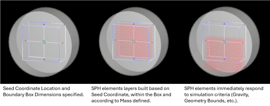
TIPS FOR USING VOLUMETRIC INLET
If desired, you can combine the usage of the imported geometries and the bounding box to achieve flat surfaces.
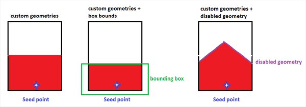
In the first image in the example above, you can see the SPH elements bed that is generated when the walls are used as the imported geometry for the Volumetric Inlet. In the second image, you can see what happens if you use the same imported geometry but add a bounding box that limits the elements generation. As the elements reach the bounding box, FreeFlow cannot inject more elements, and the surface of the Volumetric Inlet is flat.
If you want to limit the inlet to a surface that is not flat, you can use the following workaround:
Import a geometry representing the profile of your desired top surface-such as the peak used in the third image in the example above.
Set this geometry to be used only the initialization period-which is when the volume fill happens. You can accomplish this by setting the geometries Enable Time to be a very large value that ever be reached in the simulation, such as 999 s.
Before you can process your simulation, you must create at least one fluid inlet and provide either the Mass Flow Rate value or Mass value (for Volumetric Inlet).
INLETS AND OUTLETS AND EXTERNAL MODULES
If you have enabled one or more external Modules that affect your Inlet or Outlet settings, you might also have a separate Modules sub-tab or separate, module-specific settings that you can define. Refer to the Module's documentation (if provided) for more information.
INLETS AND OUTLETS PARAMETER DEFINITIONS
Use the figures and tables below to help you understand the various parameters you can set for inlets.
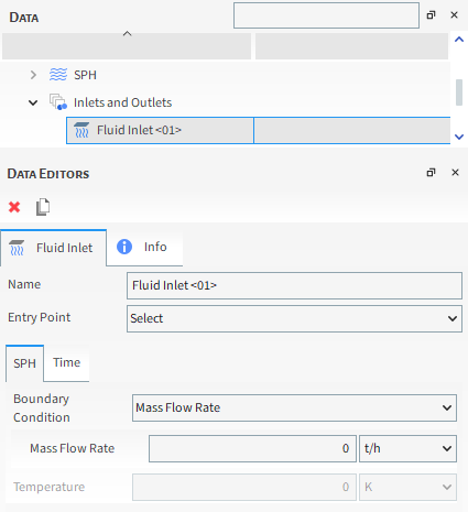
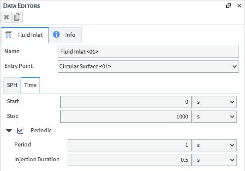
Table 3.7: Fluid Inlet parameter options
| Setting | Description | Range |
|---|---|---|
| Name |
Enables you to specify a unique identifier for the fluid inlet. | 99 character limit |
| Entry Point | The surface inlet from which the fluid is released during the
simulation. Note: Only one Inlet can be set per Entry Point. | Any Planar Surface |
| SPH | ||
| Mass Flow Rate | The mass flow rate for the SPH elements that you want released from an Entry Point | Values above but not equal to 0 kg/s. Note: The one exception to this rule is if you want to change the active Inlets after you save a copy of a partially processed pimulation for pestart purposes. |
| Velocity | The velocity for the SPH elements that you want released from an Entry Point | Values above but not equal to 0 m/s. Note: The one exception to this rule is if you want to change the active Inlets after you save a copy of a partially processed pimulation for pestart purposes. |
| Temperature | When Thermal Model is enabled this is the temperature that all SPH elements will have when released from an Entry point. | Values above but not equal to 0 K (zero Kelvin) |
| Time sub-tab | ||
| Start | The time you want fluid elements to begin releasing from the Entry Point. | Positive values Note: Check the Status panel to ensure that any variables or mathematical functions you might use results in valid values. |
| Stop | The time you want fluid elements to stop releasing from the
Entry Point. Note: If you choose to use parametric expressions in this field, know that only the resulting value and not the variables and/or mathematical functions you enter will be retained in any project copies you save for restart purposes. | Positive values Note: Check the Status panel to ensure that any variables or mathematical functions you might use results in valid values. |
| Periodic | Enables the Time Periodic control for SPH Fluid Inlets, creating a series of inlets to mimic periodic behavior. | Enable or Disable |
| Period | Defines the Time of the all period will last. | Positive values |
| Injection Duration | Defines the fluid injection duration in the already defined. | Positive values |
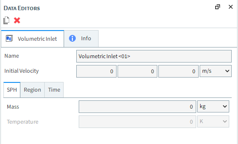
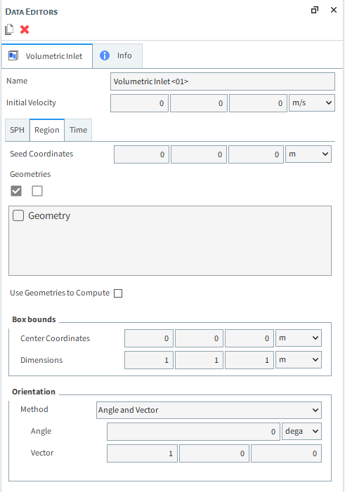
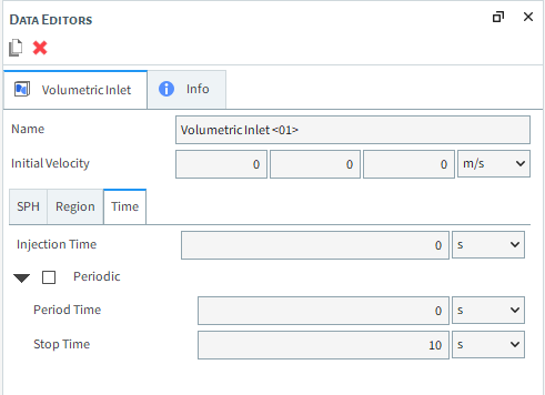
Table 4: Volumetric Inlet parameter options
|
Setting |
Description |
Range |
|---|---|---|
|
Name |
Enables you to specify a unique identifier for the inlet. |
99 character limit |
| Initial Velocity | Enables you to set a vector of initial velocities in the x, y and
z-axis for SPH elements. Important: The initial velocities vector is the same for all SPH elements defined on the same volumetric inlet. Note: The initial velocities vector cannot be changed for resume or restart simulations. | Any values |
|
SPH sub-tab | ||
|
Mass |
The target mass of fluid within the set that you want built around the Seed Coordinate, which is itself specified on the Region sub-tab. Tip: To avoid entering a value that is too large to fully simulate, ensure that you are entering a Mass value appropriate for the box volume you specify on the Region sub-tab. |
Values above but not equal to 0 kg |
|
Temperature |
When Thermal Model is enabled (see also About Physics Parameters), this is the temperature that the fluid elements will have when injected from this inlet method. |
Values above but not equal to 0 K (zero Kelvin) |
|
Region sub-tab | ||
|
Seed Coordinates |
The X, Y, and Z coordinate location of the point ("Seed") around which the SPH element layers will be built. Tip: To avoid SPH elements generation issues, ensure that you locate your Seed Coordinate away from the boundaries of your simulation geometries. |
No limit but the location must be within the limits of the Volumetric Inlet Box bounds |
|
Geometries |
Lists the imported geometry components within the simulation by which you are able to constrain your Volumetric Inlet. Specifically:
|
Turns off or on |
|
Use Geometries to Compute |
When one or more geometry components are selected from the Geometries list, selecting this option enables FreeFlow to automatically define the Box bounds based upon the limits of the selected geometries. When this option is cleared, FreeFlow will use the Box bounds you define. |
Turns off or on |
|
Box bounds Center Coordinates |
When the Use Geometries to Compute check box is cleared, this defines the X, Y, and Z coordinate location of the boundary box's center point. (The bounds of this box is what will constrain your Volumetric Inlet.) |
No limit |
|
Box bounds Dimensions |
When the Use Geometries to Compute check box is cleared, this defines the X, Y, and Z dimensions of the box that will constrain your Volumetric Inlet. |
No limit |
| Orientation Method |
Enables you to select how you want to define the orientation of the Volumetric Inlet. Specifically:
| Angle and Vector; Basis Vectors; Angles |
| Orientation Method Angle and Vector | ||
| Angle | When Angle and Vector is selected for Orientation, this is the angle the Volumetric Inlet will rotate around the Vector defined. | Any value |
| Vector | When Angle and Vector is selected for Orientation, these are the X, Y, and Z components that define the vector around which the Volumetric Inlet will rotate, using the Angle defined. | No limit but the values entered will be normalized |
| Orientation Method Basis Vectors | ||
| X-Direction | When Basis
Vectors is selected for Orientation, this is
the coordinate value defining the first of three directional vectors
that together define the final orientation of the Volumetric Inlet. Tip: To ensure correct results, make sure you define this vector as orthogonal (perpendicular) to the other two vectors. | No limit but the values entered will be normalized |
| Y-Direction | When Basis
Vectors is selected for Orientation, this is
the coordinate value defining the second of three directional
vectors that together define the final orientation of the Volumetric Inlet. Tip: To ensure correct results, make sure you define this vector as orthogonal (perpendicular) to the other two vectors. | No limit but the values entered will be normalized |
| Z-Direction | When Basis
Vectors is selected for Orientation, this is
the coordinate value defining the third of three directional vectors
that together define the final orientation of the Volumetric Inlet. Tip: To ensure correct results, make sure you define this vector as orthogonal (perpendicular) to the other two vectors. | No limit but the values entered will be normalized |
| Orientation Method Angles | ||
| Order | When Angles is selected for Orientation, this defines the order in which the three Rotation text fields will be applied. | XYZ; XZY; YXZ; YZX; ZXY; ZYX |
| Local Angles |
When Angles is selected for Orientation, this defines what coordinate system will be used as a basis for the angle specified. Specifically:
| Turns on or off |
| Time sub-tab | ||
| Injection Time | The simulation time at which you set the volumetric injection to occur. | Positive Values |
| Periodic | Enabled periodic volumetric injection of Fluid into the simulation. | Turns on or off |
| Period Time | The period at which you set the volumetric injection to occur. | Positive Values |
| Stop Time | The simulation time at which you set the periodic injection to stop. | Positive Values |
| Periodic | Enables periodic injection of Fluid. | Turns off or on |
| Period Time | Period duration. | No limit |
| Stop time | The time when Periodic injection is disabled. | No limit |
|
Modules sub-tab | ||
|
(Varies) |
These settings are specific to only certain external Modules and are therefore not documented in the FreeFlow User Manual. Refer to the Module's documentation (if provided) for more information. |
(Varies) |
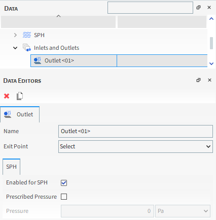
Table 6: Outlet parameter options
|
Setting |
Description |
Range |
|---|---|---|
|
Name |
Enables you to specify a unique identifier for the outlet. |
99 character limit |
|
Exit Point |
The surface that will act as an exit point for fluids during the simulation. |
Any Planar Surface |
|
SPH sub-tab | ||
|
Enabled for SPH |
Specifies if the outlet will act as an Exit Point for Fluid. |
Turns off or on |
|
Prescribed Pressure |
Specifies if the outlet will use a Prescribed Pressure as a boundary condition. |
Turns off or on |
|
Pressure |
Defines the pressure that will be applied to the Prescribed Pressure boundary condition. |
Any Value |
What would you like to do?
From the Data panel, click Inlets and Outlets, and the from the Data Editors panel, click the Create Fluid Inlet button. A new Fluid Inlet component appears under Inlets and Outlets in the Data panel.
Tip: You may also access this functionality from the right-click menu on the Data panel.
From the Data panel, click the Fluid Inlet component you just added and then from the Data Editors panel, on the main Fluid Inlet tab, enter the Name and set the Entry Point you want.
From the SPH sub-tab, do all of the following:
Set the Mass Flow Rate at the inlet.
If applicable, specify the fluid Temperature at the inlet.
From the Time sub-tab, define what you want for Start and Stop times.
See Also:
From the Data panel, click Inlets and Outlets, and the from the Data Editors panel, click the Create Volumetric Inlet button. A new Volumetric Inlet component appears under Inlets and Outlets in the Data panel.
Tip: You may also access this functionality from the right-click menu on the Data panel.
From the Data panel, click the Volumetric Inlet component you just added and then from the Data Editors panel, on the main Volumetric Inlet tab, enter the Name you want.
To add Fluid: From the SPH sub-tab, do the following:
Set the total fluid Mass.
If applicable, specify the fluid Temperature.
From the Region sub-tab, do the following:
Next to Seed Coordinates, enter the X, Y, and Z coordinate location of the spherical point around which your Volumetric Inlet layers will be built. Important: This must be located within your Box bounds.
Tip: Avoid locating this directly on the boundaries of your simulation geometries.
Do one of the following:
To have FreeFlow automatically calculate your Box bounds based upon one or more imported geometries in your simulation, select the geometries you want from the Geometries list, and then select the Use Geometries to Compute check box.
To define your own box bounds but still have your Volumetric Inlet constrained to one or more geometry components, select the geometries you want from the Geometries list, and then define the Center Coordinates and Dimensions of your Box bounds.
To define your own Box bounds and have your Volumetric Inlet ignore any geometries within the bounds you define, keep both the Geometries and the Use Geometries to Compute check boxes cleared, and then define the Center Coordinates and Dimensions of your Box bounds.
To define your Volumetric Inlet Orientation, keep the Use Geometries to Compute checkbox cleared, then select the Method and specify parameters.
If you have enabled a Module that has unique Input properties (see also About Modules Parameters), select the Modules sub-tab, and then enter the value you want for the module-specific parameters provided.
Tips:
For the Region tab:
To visualize the Box bounds and Seed location of your Volumetric Inlet input, select or create a 3D View window and then from the Data panel, select the Volumetric Inlet entity you want to see.
In the 3D View window, you can also move and resize the fill area by clicking and dragging the handles (colored dots) representing the center, and the local X, Y, and Z locations respectively.
Note: You still must move the Seed location by using the Seed Coordinates.
To see an estimate of the number of SPH elements that might be released from a Fluid Input during the simulation, view the Info tab.
Note: Ensure that the estimate includes enough elements. Volumetric Inlets require a minimum of 3 elements in order to create the "Seed".
See Also:
From the Data panel, click Inlets and Outlets, and the from the Data Editors panel, click the Create Outlet button. A new Outlet component appears under Inlets and Outlets in the Data panel.
Tip: You may also access this functionality from the right-click menu on the Data panel.
From the Data panel, click the Outlet component you just added and then from the Data Editors panel, on the main Outlet tab, enter the Name and set the Exit Point you want.
From the SPH sub-tab, do all of the following:
a. Clear the Enabled for SPH if you do not want fluid to be able to leave the simulation through this outlet. By default the check box is checked.
b. Select if you want to use a Prescribed Pressure boundary condition at the outlet.
c. If the Prescribed Pressure option was selected, define the pressure that you want prescribed at this outlet.
See Also:
From the Data panel, click the Inlet or Outlet you want to edit, and then from the Data Editors panel, modify the settings as desired.
See Also:
From the Data panel, click the Inlet or Outlet you want to remove, and then from the Data Editors panel, click the Remove button.
See Also:
Domain settings enable you to define Coordinate Limits and, if desired, an additional Periodic Domain for your simulation project.
Coordinate Limits determine where in the simulation calculations may occur. This means that any items that fall outside the limits you have defined, including SPH elements and geometries, will not be included in the simulation calculations.
For SPH elements, falling outside the coordinate limits also means they will not be visualized. For SPH elements that are set to be released outside the coordinate limits, this means they will not appear in the simulation at all. For SPH elements that were within the limits but then exited out of them, this means those SPH elements will disappear immediately upon leaving the limits (Figure 3.70: SPH element's behavior when exiting the coordinate limits).
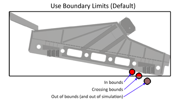
For geometries, falling outside the coordinate limits means only that they are not included in calculations. Geometries will still be visualized regardless of whether or not they are within the coordinate limits.
Because of these reasons, it is important that you set your coordinate limits appropriately for the type of simulation you are setting up. For closed systems, such as mixers and mills, where SPH elements are not expected to fall outside of the geometry limits, choosing to use the Use Boundary Limits check box might be the best option.
For open systems, where SPH elements are expected to reach beyond the limits of the geometries, setting your own custom coordinate limits might be a better option.
Periodic Domains enable you to include an additional domain within your simulation Coordinate Limits within which SPH elements that are exiting out one side of the periodic domain area are recycled back into the domain from the opposite side.
In this version of FreeFlow, periodic domains can either be Cartesian, which are based upon two parallel planes (box-shaped domain), or Cylindrical, which are based upon two intersecting planes rotated by an angle to create a cylindrical sector (wedge-shaped domain).
Both types of periodic domains do not allow the injection of SPH elements outside the bounds of the periodic domain. This means that when setting up your SPH Inputs, ensure that your Fluid Inlet or Volumetric Inlet box bounds definitions are located well within your periodic domain. (See also About Adding and Editing Inlets and Outlets.)
ABOUT CARTESIAN PERIODIC DOMAINS
Cartesian Periodic Domains are the original type of what used to be known as "periodic boundaries" and whose functionality has been included with FreeFlow since its earliest releases. When choosing to use Cartesian Periodic Domains, two parallel planes are created along the axis (or combination of axes) you specify. SPH elements that exit the simulation through one plane will reappear in the simulation through the opposite plane (Figure 3.71: SPH elements behavior when exiting only the coordinate limits (left) and then with a periodic cartesian domain set (right)).
Figure 3.71: SPH elements behavior when exiting only the coordinate limits (left) and then with a periodic cartesian domain set (right)
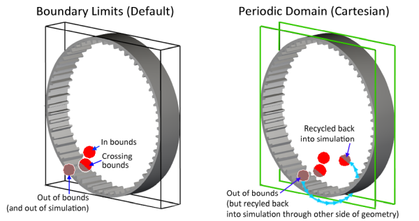
This is especially useful for simulating cross sections. SPH elements flung out of one side of domain can be recycled back into the simulation from the other side.
Tip: If you choose to set Cartesian periodic domains, ensure that the periodic domain width (the distance between the Min Coordinate and Max Coordinate values) is at least 5 times wider than the largest SPH element size, when opting for Wendland or Cubic Kernel Type. Or, alternatively, ensure that your largest SPH element size is less than 0.2 times the width of your periodic domain. For Quintic Kernel Type, ensure that the periodic domain width is at least 7.5 times wider than the largest SPH element, or make sure that the largest element is less than 0.13 times the widht of the periodic domain.
For example, a 0.1 m SPH element can work in a 0.5 m or wider periodic domain. Alternatively, a 1 m periodic domain can support a 0.2 m or smaller SPH element size.
Note: FreeFlow's Cartesian Periodic Domain functionality was originally designed to be located at the extreme ends of the geometry in question, for example, at the limits of a Mill slice. Sometimes, however, it is desirable to make your periodic domain smaller than the geometry and/or coordinate limits of the domain. FreeFlow will support you doing this, but be aware that depending on the configuration of the geometries and the periodic limits, it is possible that during the simulation, some SPH elements might go through the walls of your geometries in an unexpected manner.
Important: As shown in the figure Figure 3.72: Geometry triangles lying fully on the periodic plane (in green) should be removed or disabled. For simulations where the geometry motion is in the periodic plane (For example, if the periodic direction is Z then the periodic plane is X-Y. If the periodic direction is Y then the periodic plane is X-Z. If the periodic direction is X then the periodic plane is Y-Z.), any triangles whose all 3 vertices exactly lie on the periodic plane should either be removed from the geometry design in a CAD tool prior to being imported into FreeFlow, or be disabled by FreeFlow to ensure proper simulation results. In this version of FreeFlow, these triangles are disabled for you by default. (See also About Solver Parameters.)
Figure 3.72: Geometry triangles lying fully on the periodic plane (in green) should be removed or disabled
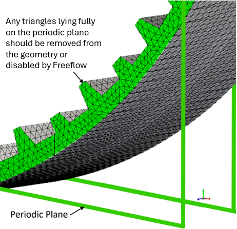
ABOUT CYLINDRICAL PERIODIC DOMAINS
Similar to Cartesian Periodic Domains, Cylindrical Periodic Domains enable you to specify the locations of two planes between which SPH elements are recycled. But rather than being parallel, the two planes in a Cylindrical Periodic Domain are intersecting and rotated by an angle, creating a cylindrical sector, which can look similar in shape to a "wedge" or "slice" of pie.
This can be useful in cylindrical mixing devices, for example, where simulating only a slice of the device would have similar SPH element properties as simulating the full device, but with many fewer elements and calculations.
The size of the wedge is determined by the number of (evenly spaced) radial divisions you specify for the cylinder. So a division of 2 would create a wedge half the size of the cylinder. A division of 3 would create a wedge a third the size of the cylinder, and so on.
The placement of the wedge is determined both by the location of the cylinder, which is orientated along the X, Y, or Z Periodic Direction you specify, and the Initial Angle value you specify for the first plane, which will be measured in the positive plane perpendicular to the Periodic Direction.
Tip: The positive angular direction is always counterclockwise when the Periodic Direction is set to point towards outside the screen (top view). This means:
For a Periodic Direction of Y, the Initial Angle is measured from the positive Z axis
For a Periodic Direction of X, the Initial Angle is measured from the positive Y axis
For a Periodic Direction of Z, the Initial Angle is measured from the positive X axis
In the mixing drum example shown in the image below (Figure 3.73: Illustration of how the size and location of a Cylindrical Periodic Domain is
determined), the Periodic
Direction is Y, the Initial Angle is 30 degrees, and the Number of Divisions is 3. These
settings result in a periodic, wedge-shaped domain (area in red) that begins 30
degrees counterclockwise in the positive Z direction, and ends 120 degrees (360/3
divisions) later.
Figure 3.73: Illustration of how the size and location of a Cylindrical Periodic Domain is determined

LIMITATIONS AND BEST PRACTICES
When setting a Cylindrical Periodic Domain, keep in mind the following requirements, limitations, and best practices:
The Periodic Direction must be aligned with one of the three main axes (X, Y, or Z) and must also be parallel to the gravity direction you have set for the simulation.
Because the size of the wedge is determined by how many (evenly spaced) radial divisions you specify, the Number of Divisions value must be a whole integer equal to 2 or greater.
Your Fluid Inlet or Volumetric Inlet box bounds definitions must be located within the limits of the periodic domain.
It is recommended that you design your geometries, define your SPH element size, and set your Cylindrical Periodic Domain limits such that your periodic domain width (the distance between the periodic planes) at any radial distance from the origin is at least 5 times wider than the element size. As illustrated on the left side of Figure 3.74: Cylindrical Periodic Domain with full wedge (left) and with center removed (right), in most cases, elements at the narrowest part of the wedge will not meet these requirements, which is likely to cause instabilities and affect the accuracy of the results. It is therefore recommended that you apply Cylindrical Periodic Domains only to elements that are simulated in a ring shape, similar to when you specify a Cylinder User Process with the Hole defined (right side of Figure 3.74: Cylindrical Periodic Domain with full wedge (left) and with center removed (right)).
To reduce the chance of simulation errors, ensure that your geometry triangles fall inside the selected domain and that the periodic planes do not cross the triangle surfaces. The ideal situation is to have the periodic planes crossing along the exact edges of the triangles, as shown on the right side of Figure 3.75: Periodic Planes intersecting Boundary Triangles (left) and aligning on the edges (right).
Figure 3.75: Periodic Planes intersecting Boundary Triangles (left) and aligning on the edges (right)
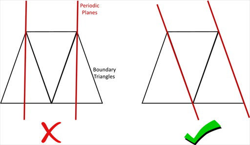
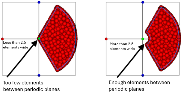
DOMAIN SETTINGS PARAMETER DEFINITIONS
Use the figures and table below to help you understand the various Domain Settings parameters you can set for a simulation project.
Figure 3.76: Domain Settings, Coordinate Limits parameters in the Data Editors panel (No periodic domain)
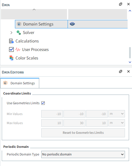
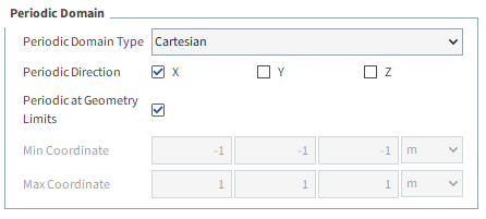
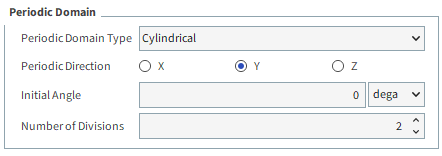
Table 1: Domain Settings parameter options
|
Setting |
Description |
Range |
|---|---|---|
|
Coordinate Limits | ||
|
Use Geometries Limits |
When selected, automatically sets the coordinate limits of the simulation at the extreme ends of the existing geometries. When geometries change or move, the limits will be changed also. Notes:
|
Turns on or off |
|
Min Values |
When Use Geometries Limits is cleared, this enables you to set the minimum values for the simulation coordinate limits in the following format: X Y Z These custom limits will be visible in the 3D View. |
No limit for X, Y, and Z values but must be lower than Max Values |
|
Max Values |
When Use Geometries Limits is cleared, this enables you to set the maximum values for the simulation coordinate limits in the following format: X Y Z These custom limits will be visible in the 3D View. |
No limit for X, Y, and Z values but must be higher than Min Values |
| Reset to Geometries Limits | When the Use Geometries Limits option is disabled, Reset to Geometries Limits allows you to automatically set the Domain's minimum and maximum values to the limits of the current geometries. | |
|
Periodic Domain | ||
|
Periodic Domain Type |
Enables you to choose whether or not to include a periodic domain, and if so, what type of domain you want to include. Specifically:
|
No periodic domain; Cartesian; Cylindrical |
|
Periodic Direction |
When either Cartesian or Cylindrical is selected as Periodic Domain Type, this determines the direction periodic domains are enabled. Specifically:
|
Turns on or off |
|
Periodic at Geometry Limits |
When Cartesian is set for Periodic Domain Type, enabling this check box locates the periodic domain at the farthest edge of the simulation geometries. When cleared, the Min. Coordinate and Max. Coordinate values will be used to define the periodic domain limits. |
Turns on or off |
|
Min Coordinate |
Location along the axis specified for Periodic Direction to place the first of two planes that define the box-like shape of the cartesian periodic domain limits. Tip: Ensure the distance from this coordinate to the Max Coordinate is at least 5 times wider than the largest SPH element size. |
No limit |
|
Max Coordinate |
Location along the axis specified for Periodic Direction to place the second of two planes that define the box-like shape of the cartesian periodic domain limits. Tip: Ensure the distance from this coordinate to the Min Coordinate is at least 5 times wider than the largest SPH element size. |
No limit |
|
Initial Angle |
When Cylindrical is set for Periodic Domain Type, this determines the location of the first of two intersecting planes that define the wedge-like shape of the cylindrical periodic domain limits. How this value is measured depends upon the Periodic Direction specified. Specifically:
Entering a 0 (zero) value will align the first plane with the axis of measure. Entering any other value will offset the plane by that angle amount. |
No limit |
|
Number of Divisions |
When Cylindrical is set for Periodic Domain Type, this defines how the cylinder will be divided to determine the final size of the wedge. Specifically:
|
Whole numbers greater than or equal to 2 |
What would you like to do?
See Also:
Unlike most setup parameters, which you can define only prior to processing, you are able to change the parameters under Execution on the Solver | General tab, or any of the options on the Solver | Advanced tab after processing has started without invalidating your results. You must first Stop processing, change the parameters you want, and then Resume processing again in this scenario. (See also I cannot change my setup parameters during processing .)
Use the figures and tables below to help you understand the various Solver parameters you can set for a simulation project.
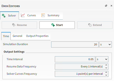
Table 1: Solver | Time parameter options
|
Setting |
Description |
Range |
|---|---|---|
|
Simulation Duration |
The total amount of real time that you want the simulation to run. Tip: When calculating the Simulation Duration value, be sure to account for the mass flow rate of your SPH elements, steady-state, and so on. |
Positive values |
|
Output Settings Time Interval |
The time intervals at which you want your output files to be saved. Tip: To prevent rotating or vibrating boundaries from appearing like they are moving backwards, divide the rotational velocity (for rotating boundaries) or frequency (for vibrating boundaries) by 2 and then set your simulation output frequency as slightly lower than that value. Tip: FreeFlow also has a feature to select multiple output frequencies during the simulation, which is useful to increase or reduce the output data after some time, so that specific phenomena can be evaluated with more or less detail. |
Value must be positive but less than Simulation Duration |
|
Output Settings Solver Curves |
Controls the frequency at which the Solver Curves are updated while the simulation is being processed. The value entered here represents the number of times the Solver Curves will be updated between two consecutive outputs. For example, if the Simulation Output Settings is set to 1 [s] and the Solver Curves Output Frequency is set to 100, it means that the Solver Curves will be updated at every 0.01 [s]. Note: FreeFlow will limit the time interval for updating the Solver Curves Frequency to be larger than 100 simulation time steps. |
Whole values greater than zero |
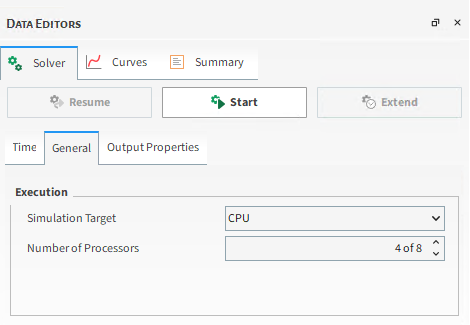
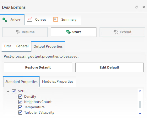
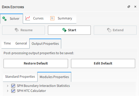
|
Output Properties |
Description |
Range | |
|---|---|---|---|
| Properties |
SPH |
Select all SPH properties that can be used in the post-processing |
Turns on or off |
| Geometries |
Select all Geometries properties that can be used in the post-processing |
Turns on or off | |
|
CFD |
Select all CFD properties that can be used in the post-processing |
Turns on or off | |
| Module Properties |
SPH Boundary Interaction Statistics |
Select all SPH Boundary Interaction Statistics properties that can be used in the post-processing |
Turns on or off |
|
SPH HTC Calculator |
Select all SPH HTC Calculator properties that can be used in the post-processing |
Turns on or off | |
What would you like to do?
See Also:
User Processes are the tools available in FreeFlow to help you analyze a simulation after it has been processed, allowing you to focus on specific views or data you want to analyze, by using different planes, shapes and filters. This way, it is possible to divide, reduce and/or filter the simulation results and gather the desired information.
This section will mainly focus on presenting the various forms of User Processes and where they are located. Further information on the use of User Processes and Simulation Analysis are available in the "Analyzing a Simulation" Chapter. There you will find all information necessary on the use of User Processes.
The Image below clarifies how a User Process is activated. This applies to every entity that allows the creation of User Processes.
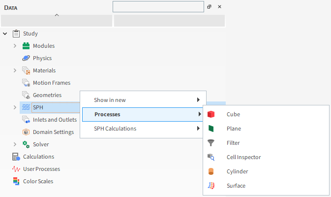
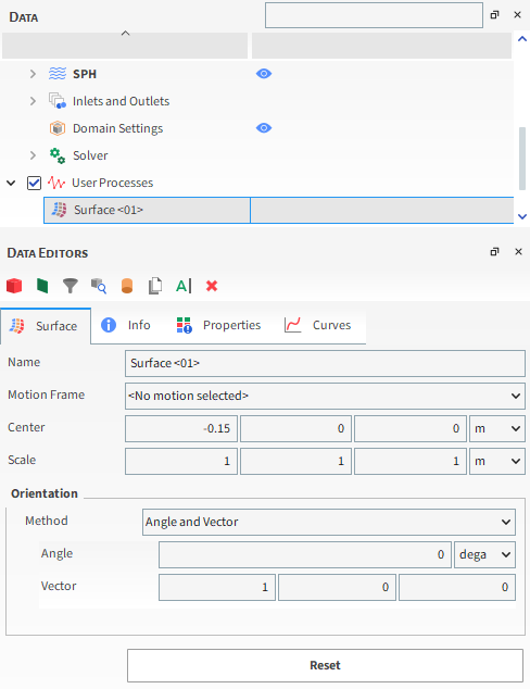
Note: When a User Process is selected, the entity upon which it was created is also highlighted.
Table 3.8: User Processes Basic Description
| User Process | Description |
|---|---|
| Cube |
You can define, within the simulation boundaries, a three dimensional analysis box of whatever length, width, and height desired. |
| Plane | You can limit the analysis area of the simulation based upon a user-defined plane, by either viewing all of the results behind the plane, or limiting the results to only the data immediately surrounding the plane. |
| Filter | You can limit the simulation results by a certain property. This way, it is possible to focus the selection to only the calculation and data ranges you want. |
| Cell Inspector |
You can select and inspect the details of an individual cell making up a particular entity, by applying it to specific simulation entities. |
| Cylinder |
You can define, within the simulation boundaries, a three dimensional analysis tube, arch, or slice of whatever diameter and height desired, and with or without a center hole. |
| Surface |
You can import a custom .stl surface, which then can be used to measure SPH mass flow rate in post-processing phase. |
| Streamlines | You can use Streamlines to analyze the flow patterns or
trajectories of SPH elements in a simulation. The concept of streamlines in SPH is similar to that in traditional fluid dynamics. Streamlines represent the paths that individual fluid elements would follow in the flow field. |
Table 3.9: User Processes available by Entity
|
Entity |
Available User Processes |
|---|---|
|
Geometries | |
| Wall |
Cube, Plane, Filter, Cell Inspector and Cylinder |
| Imported Surface |
Cube, Plane, Filter, Cell Inspector and Cylinder |
| System Coupling Wall |
Cube, Plane, Filter, Cell Inspector and Cylinder |
|
SPH |
Cube, Plane, Filter, Cell Inspector and Cylinder, Surface |
| Eulerian Solution |
Cube, Plane, Filter, Cell Inspector and Cylinder, Streamlines |
| User Processes | |
| Cube, Plane, Filter, Cylinder, Surface and Streamlines |
All of the User Processes referenced on the left allow you to create another User Process upon them. For example: you are able to create a Cube User Process to define a specific region of the simulation and then create a Filter User Process upon said Cube, making it possible to analyze a fluid property in a user-defined region. |
| Cell Inspector |
The Cell Inspector is a User Process you can apply to specific simulation entities that enables you to select and inspect the details of an individual cell making up that particular entity. It is not possible to create another User Process upon the Cell Ispector. |
See Also:
Coloring a simulation entity by a certain property is a useful tool in post-processing analysis. Some examples, are: coloring a moving fluid by velocity, or a static fluid by pressure. Which makes the analysis process much more visible for the user.
This section focuses mainly on presenting Color Scales. Further information on the use of Color Scales and Simulation Analysis are available in the "Analyzing a Simulation" Chapter. There you will find all necessary information on the use of Color Scales.
The sequence of Images below clarifies the activation and use of Color Scales.
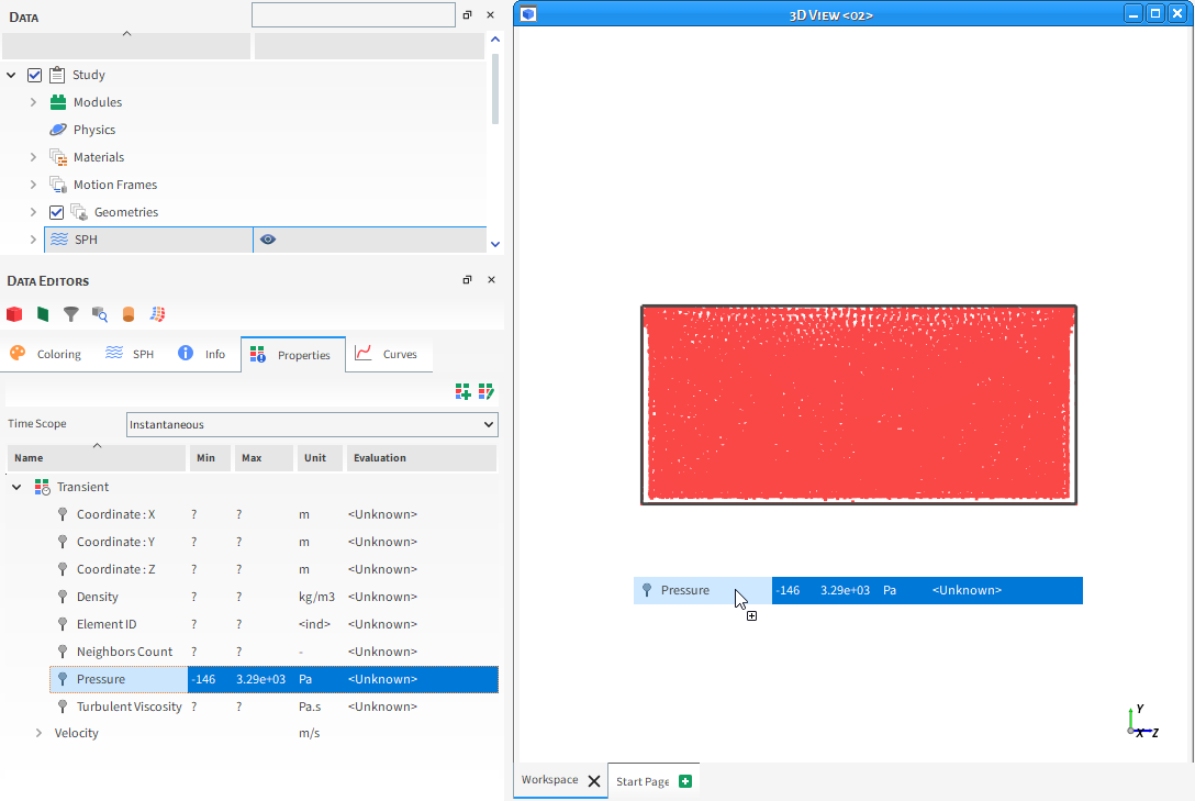
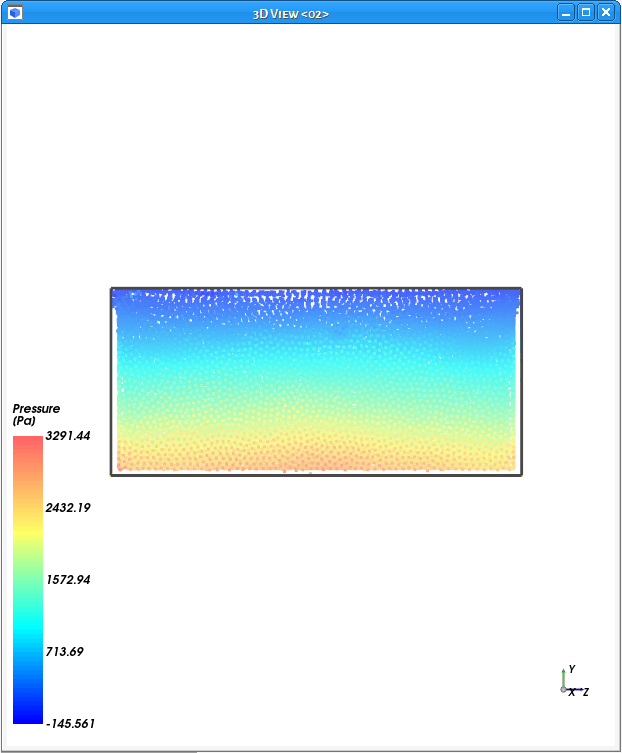
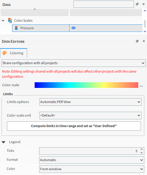
What would you like to do?
The SPH feature has a support for Region of Interest (ROI). This means that it is capable of freezing and disabling SPH-SPH interactions outside a given region. With this feature, there can be a simulation speed increase.
Regions of Interest enable you to specify an area inside the simulation domain within which certain external Modules can perform custom calculations.
Tip: Unless you have enabled an external Module that makes use of a Region of Interest, you can skip this part of your FreeFlow setup.
What would you like to do?
See Also:
A Region of Interest (sometimes referred to as a "ROI") enables you to specify an area inside the simulation domain within which certain external Modules can perform custom calculations. The calculations within this "sub-domain" results in data that can be visualized and analyzed through other entities—such as SPH elements and Geometries—similar to how calculations in the main domain function.
Tip: Unless you have enabled an external Module that makes use of a Region of Interest, you can skip this part of your Feeflow setup.
In this version of FreeFlow, there are two shape options you can define as a Region of Interest:
A Cube, which enables you to create a box-like shape.
A Cylinder, which enables you to create a full or partial cylindrical shape, with or without a center hole.
While both shapes have setups and appearances similar to those of their User Process cousins (see also About User Processes Parameters), a Region of Interest shape is quite different in purpose and function as illustrated in Figure 3.88: Comparison of a User Process Shape with a Region of Interest Shape.
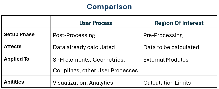
What would you like to do?
See Also:
The Cube Region of Interest enables you to define within the simulation boundaries a three dimensional box of whatever length, width, and height you want. In this way, you can limit the calculations of certain external Modules to only the domain selection contained within the box.
Tip: Unless you have enabled an external Module that makes use of a Region of Interest, you can skip this part of your FreeFlow setup.
Like Cube User Processes, you can use the colored directional handles (Figure 3.89: Cube Region of Interest during project setup) in a 3D View window to change the shape and location of the box, or you can define exact values in the Data Editors panel.
See the image and table below to learn more about the Cube Region of Interest.
CUBE REGION OF INTEREST PARAMETER DEFINITIONS
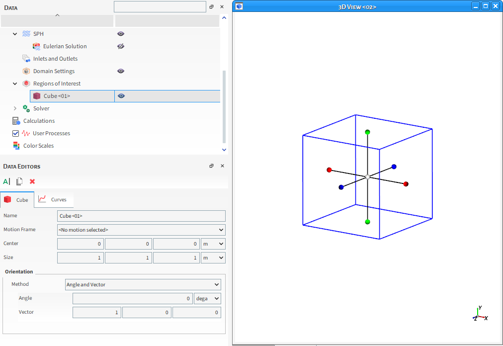
Table 1: Cube Region of Interest Parameter Options
|
Setting |
Description |
Range |
|---|---|---|
|
Name |
Enables you to specify a unique identifier for the Region of Interest. Note: This same name will appear in the Data panel under Regions of Interest. |
No limit |
|
Center |
The X, Y, and Z coordinate locations of the cube's center point. |
Any value |
|
Size |
The length of the cube's three sides as specified in the X, Y, and Z directions. |
Any value |
| Orientation | ||
|
Method |
Enables you to select how you want to define the orientation of the cube shape. Specifically:
|
Angles; Angle and Vector; Basis Vectors |
|
Method Angles | ||
|
Order |
When Angles is selected for Orientation, this defines the order in which the three Rotation text fields will be applied. |
XYZ; ZXY; YXZ; YZX; ZXY; ZYX |
|
Local Angles |
When Angles is selected for Orientation, this defines what coordinate system will be used as a basis for the angle specified. Specifically:
|
Turns on or off |
|
Rotation |
When Angles is selected for Orientation, this is the degree of cube rotation in each of the three directions specified by the Order provided. |
Any value |
|
Method Angle and Vector | ||
|
Angle |
When Angle and Vector is selected for Orientation, this is the angle the cube will rotate around the Vector defined. |
Any value |
|
Vector |
When Angle and Vector is selected for Orientation, this is the X, Y, and Z components that define the vector around which the cube will rotate, using the Angle defined. |
No limit but the values entered will be normalized |
|
Method Basis Vectors | ||
|
X direction |
When Basis Vectors is selected for Orientation, this is the coordinate values defining the first of three directional vectors that together define the final orientation of the cube. Tip: To ensure correct results, make sure you define this vector as orthogonal (perpendicular) to the other two vectors. |
No limit but the values entered will be normalized |
|
Y direction |
When Basis Vectors is selected for Orientation, this is the coordinate values defining the second of three directional vectors that together define the final orientation of the cube. Tip: To ensure correct results, make sure you define this vector as orthogonal (perpendicular) to the other two vectors. |
No limit but the values entered will be normalized |
|
Z direction |
When Basis Vectors is selected for Orientation, this is the coordinate values defining the third of three directional vectors that together define the final orientation of the cube. Tip: To ensure correct results, make sure you define this vector as orthogonal (perpendicular) to the other two vectors. |
No limit but the values entered will be normalized |
What would you like to do?
See Also:
The Cylinder Region of Interest enables you to define within the simulation boundaries a three dimensional analysis cylinder, arch, or slice of whatever radius and height you want, and with or without a center hole. (See Figure 3.90: Cylinder arc results with different Final angle values for examples.) In this way, you can limit the data an external Modules calculates to only the selection contained by the shape you determine. The method is particularly useful for analyzing certain areas of equipment with round components, such as mills and pipes.
Note: Unlike Cylinder User Processes, which can be elliptical in shape, Region of Interest Cylinders must only be perfectly round.
See the images and table below to learn more about the Cylinder Region of Interest.
Tip: You can use Colored Directional Handles to change the shape and location.
What you set for your Initial and Final Arc Angle values determine how far around the Y axis the arc for the cylinder will be drawn. Cylinder Arc Angles follow the right-hand rule: when the Y axis points outside the screen (from the Fit menu, select Camera Preset: +Y), no matter whether you enter a positive or negative value for the Final parameter, the arc will be drawn from the Initial value counterclockwise to your Final value. (See Figure 3.90: Cylinder arc results with different Final angle values below for an illustration.)
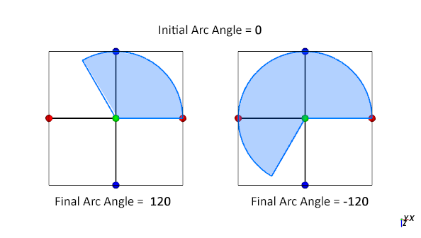
CYLINDER REGION OF INTEREST PARAMETER DEFINITIONS
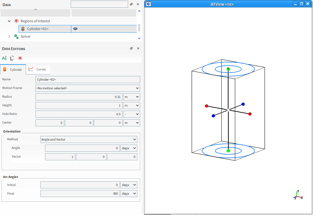
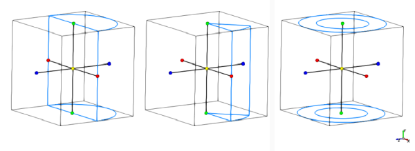
Table 1: Cylinder Region of Interest parameter options
|
Setting |
Description |
Range |
|---|---|---|
|
Name |
Enables you to specify a unique identifier for the Region of Interest. Note: This same name will appear in the Data panel under Regions of Interest. |
No limit |
|
Center |
The X, Y, and Z coordinate locations of the shape's center point. |
Any value |
|
Radius |
The size of the cylinder's outer radius. |
Any value |
|
Height |
The size of the shape's dimension in the Y direction. |
Any value |
|
Hole Ratio |
The percentage of volume that the center hole through the cylinder will take up. |
0-1 |
| Orientation | ||
|
Method |
Enables you to select how you want to define the orientation of the cylinder shape. Specifically:
|
Angles; Angle and Vector; Basis Vectors |
|
Method Angles | ||
|
Order |
When Angles is selected for Orientation, this defines the order in which the three Rotation text fields will be applied. |
XYZ; ZXY; YXZ; YZX; ZXY; ZYX |
|
Local Angles |
When Angles is selected for Orientation, this defines what coordinate system will be used as a basis for the angle specified. Specifically:
|
Turns on or off |
|
Rotation |
When Angles is selected for Orientation, this is the degree of cylinder rotation in each of the three directions specified by the Order provided. |
Any value |
|
Method Angle and Vector | ||
|
Angle |
When Angle and Vector is selected for Orientation, this is the angle the cylinder will rotate around the Vector defined. |
Any value |
|
Vector |
When Angle and Vector is selected for Orientation, this is the X, Y, and Z components that define the vector around which the cylinder will rotate, using the Angle defined. |
No limit but the values entered will be normalized |
|
Method Basis Vectors | ||
|
X direction |
When Basis Vectors is selected for Orientation, this is the coordinate values defining the first of three directional vectors that together define the final orientation of the cylinder. Tip: To ensure correct results, make sure you define this vector as orthogonal (perpendicular) to the other two vectors. |
No limit but the values entered will be normalized |
|
Y direction |
When Basis Vectors is selected for Orientation, this is the coordinate values defining the second of three directional vectors that together define the final orientation of the cylinder. Tip: To ensure correct results, make sure you define this vector as orthogonal (perpendicular) to the other two vectors. |
No limit but the values entered will be normalized |
|
Z direction |
When Basis Vectors is selected for Orientation, this is the coordinate values defining the third of three directional vectors that together define the final orientation of the cylinder. Tip: To ensure correct results, make sure you define this vector as orthogonal (perpendicular) to the other two vectors. |
No limit but the values entered will be normalized |
| Arc Angles | ||
|
Initial Arc |
The initial degree point around the Y axis that the circular portion of the cylinder will be drawn. When the Y axis points outside the screen, the resulting arc will be drawn from the initial angle counterclockwise to the final angle. Tip: To draw a full cylinder, keep this value zero (0) and set Final to 360. |
Any value |
|
Final Arc |
The final degree point around the Y axis that the circular portion of the cylinder will be drawn. when the Y axis points outside the screen, the resulting arc will be drawn from the initial angle counterclockwise to the final angle. Tip: To draw a full cylinder, set this value to 360 and keep Initial at zero (0). |
Any value |
What would you like to do?
See Also:
Ensure you have enabled an external Module that makes use of Regions of Interest.
Tip: If you do not plan to enable an external Module that makes use of Regions of Interests, then you do not need to add a Region of Interest to your simulation.
From the Data panel, right-click Study, select Regions of Interest and then create the shape you want to.
Note: The Regions of Interest entity shows up when you create a ROI, otherwise it will be hidden from the Study.
From the Data panel, select the newly created ROI below Regions of Interest, and from the Data Editors panel, on the shape tab for the item (Cube or Cylinder), enter the options you want.
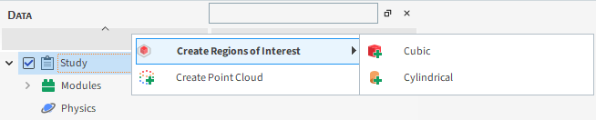
Tip: In the 3D View window, you can also move and resize the Region of Interest area by clicking and dragging the handles (colored dots).
See Also:
EDIT OR REMOVE A REGION OF INTEREST
From the Data panel, under Regions of Interest, select the entry that you want to change.
From the Data Editors panel, do one of the following:
To edit the entity, from the shape tab for the item (Cube or Cylinder), change the settings you want.
To remove the entity, click the Remove button.
See Also:
Point Clouds enable you to import a text file containing field data that defines one or more points in space.
Tip: Unless you have enabled an external Module that makes use of Point Clouds, you can skip the Point Clouds part of your FreeFlow setup.
What would you like to do?
See Also:
In FreeFlow, the primary purpose of Point Clouds are to support the functionality within custom external Modules whose models require information that varies through all three dimensions of the domain and/or over time.
Tip: Unless you have enabled an external Module that makes use of Point Clouds, you can skip the Point Clouds part of your FreeFlow setup.
Specifically, Point Clouds enable you to import a text file containing field data that defines one or more static points in space. Moreover, you can load a set of point clouds at once by importing a transient point cloud text file, which specifies the start and end times for individual static point clouds. This data can then be used by FreeFlow in various ways depending upon the functionality of the external Module making use of the Point Cloud.
(See also About Modules Parameters.)
ABOUT CREATING A STATIC POINT CLOUD DEFINITION FILE
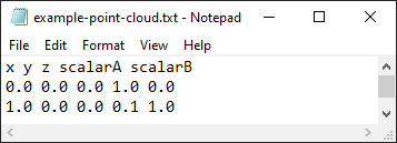
The text file you import for a Static Point Cloud must be formatted in the following way:
The file must be saved as a .txt extension with spaces separating each value. Important: No matter your system's location settings, ensure that you use dots (periods) and do not use commas to indicate decimals in this particular text file.
The first (header) row must contain the names of each value defined.
The first three (required) columns must be
(x, y,
                        z)
, which together define the coordinate location of the point.The forth (required) column must include a scalar variable. (The variable you include will be dependent upon how the Point Cloud will be used.)
The fifth and subsequent columns (optional) can include additional scalar variables as needed.
The second and subsequent rows define the values for each individual point.
ABOUT CREATING A TRANSIENT POINT CLOUD DEFINITION FILE
Figure 3.95: Example text file defining the main file of a Transient Point Cloud with three Static Point Clouds.
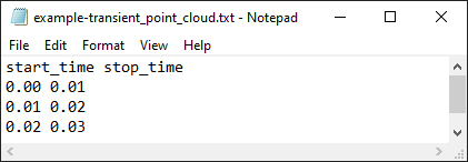
Transient Point Clouds consist of sets of Static Point Clouds that are applied during the simulation following specific start and end times. In order to import a Transient Point Cloud, it is necessary to import a main text file containing the start and end times of each Static Point Cloud that will be then automatically imported to compose the Transient Point Cloud.
The main text file you import for a Transient Point Cloud must be formatted in the following way (see Example text file defining the main file of a Transient Point Cloud with three Point Clouds):
The file must be saved as a .txt extension with spaces separating each value. Important: No matter your system's location settings, ensure that you use dots (periods) and not commas to indicate decimals in this particular text file.
The first (header) row must contain only the start_time and the stop_time names.
The second and subsequent rows define the start time and the stop time values for the Static Point Clouds that you want to be imported.
The start time value in the first row is not necessarilly required to be zero.
The stop time entry in the last row can be empty so the last Static Point Cloud will be enabled until the end of the simulation.
Figure 3.96: Example text files structure to define a Transient Static Point Cloud with three Static Point Clouds.
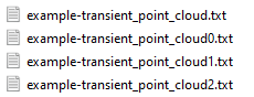
The Static Point Clouds text files that makes up the Transient Point Clouds must have the same format as the regular Static Point Clouds. (See also About Creating a Static Point Cloud Definition File.)
The Transient Point Cloud files structure must follow these rules (see Example text file defining the main file of a Transient Point Cloud with three Point Clouds):
The main Transient Point Cloud text file and each Static Point Cloud text files must be located at the same folder.
The filename of each of the Static Point Clouds must be the same one used for the main Transient Point Cloud txt file, but adding an index at the end of the filename.
The start and the stop times defined in the main text file rows will be considered to load the Static Point Clouds into the simulation. Each row is related to each Static Point Cloud index, starting from 0.
In this version of FreeFlow, you can visualize in a 3D View window the individual points defined within your Point Cloud Definition File (Figure 3.97: A Point Cloud being visualized in a 3D View window).
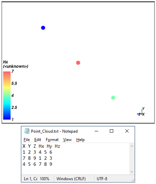
POINT CLOUD PARAMETER DEFINITIONS
Use the image and table below to help you understand the settings for a Point Cloud.
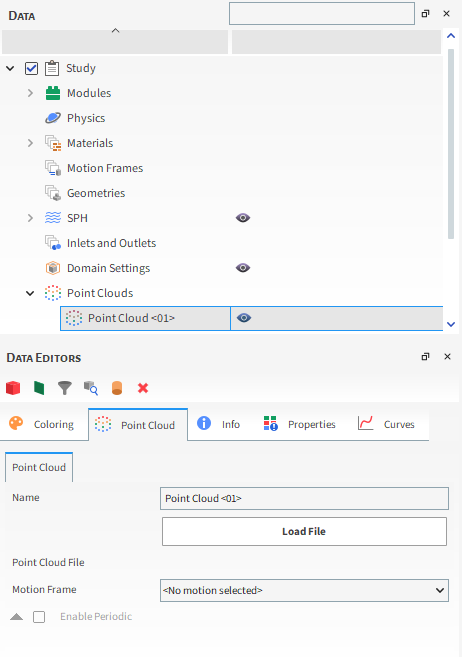
Table 1: Point Cloud parameter options
|
Setting |
Description |
Range |
|---|---|---|
|
Name |
Enables you to specify a unique identifier for the Point Cloud. |
99 character limit |
What would you like to do?
See Also:
Ensure you have enabled an external Module that makes use of Point Clouds.
Tip: If you do not plan to enable an external Module that makes use of Point Clouds, then you do not need to add a Point Cloud to your simulation.
Ensure you have a Point Cloud definition text file that is formatted according to the way FreeFlow expects. (See also About Point Clouds.)
From the Data panel, right-click Study, select Point Cloud, and then click Create Point Cloud.
From the Data panel, under Point Clouds select the newly added Point Cloud entry.
Note: The Point Clouds entity shows up only if you create a Point Cloud, otherwise it will be hidden from the Study.
From the Data Editors panel, on the main Point Cloud tab, enter a Name and then click the Load File button.
From the Select file to import dialog, navigate to and select the .txt file you want to use, and then click Open.
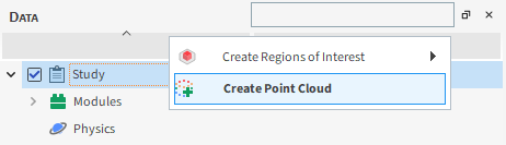
See Also:
From the Data panel, under Point Clouds select the Point Cloud entry you want to change.
From the Data Editors panel, do one of the following:
To edit the Point Cloud, from the main Point Cloud tab, do any of the following:
Enter a different Name.
Click the Load File button and then from the Select file to import dialog, navigate to and select the new .txt file you want to use, and then click Open.
To remove the Point Cloud, click the Remove Point Cloud button.
SEARCH CUT-OFF
The Search Cut-Off feature improves performance during nearest-point searches in point clouds. When enabled, the solver skips searching for neighbors that are farther than a specified physical distance, reducing computation time.
To use it, enable Search Cut-Off and set the Distance parameter to define the region where particles will be ignored. Points outside this distance will not have a valid neighbor index. Use larger distances for detailed searches and smaller ones for faster performance.
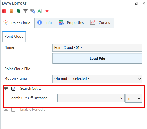
See Also:
Before you process a simulation, it is a good idea to check the key criteria provided on the Simulation Summary dialog. Doing this can help you catch data entry errors, and can help you get a rough estimate of how long the simulation might take to process.
At any point, you may also check the Summary tab on the Solver entity to gain access to the same information. From here, you can also see the FreeFlow version and simulation save dates for the project.
What would you like to do?
See Also:
Checking the key criteria listed on the Simulation Summary dialog (or tab) before you get too far into processing your simulation can help you catch data entry errors, which has the potential of saving you time in processing your simulation.
The Simulation Summary dialog automatically appears whenever you start a new simulation (see also Start Processing a Simulation from the Beginning ). You can also view similar summary information after processing has started from the Solver entity. No matter whether processing has started or not, the Summary tab is also where you can find valuable timestamp information for the project, such as in what version of FreeFlow the project was created or last saved.
If you see information on the Summary that indicates that there might be an error in your setup, for example, the Number of SPH elements is higher than expected. You can either click Cancel on the dialog, which will stop the simulation from initialization, or if the dialog has already closed, you can click the Stop button on the Solver tab in the Data Editors panel. Both actions will stop the simulation from processing so that you can review and fix your setup information before continuing.
Besides helping you pin-point potential errors, the Summary information can also act as an indicator for how long it might take your simulation to process. While a higher Time Step Duration value will typically result in a faster simulation, for all other properties provided on the Simulation Summary, higher numbers and True values will generally result in longer simulation processing times.
Tip: To verify the number of SPH elements without having to start processing the simulation, you can also view the information on the Info tab of the SPH entity at any time during your project setup.
Use the figures and table below to understand the various types of summary information provided for simulations.
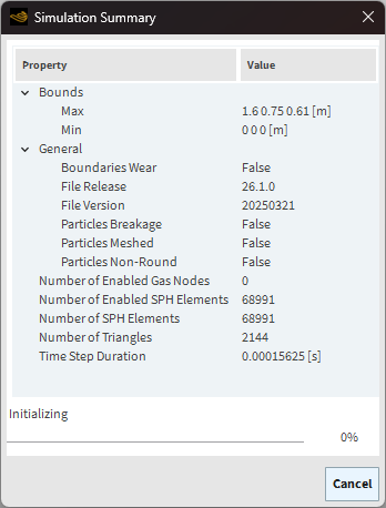
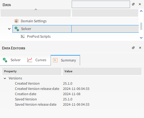
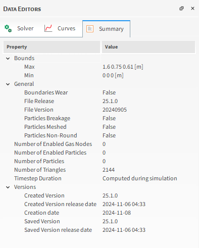
Table 1: Simulation Summary dialog and tab options
|
Property |
Description |
|---|---|
|
Bounds | |
|
Max |
The maximum coordinates for which geometry triangles are drawn. If Set as Boundary Limits is selected, once a SPH element reaches these limits, it will be removed from the calculations and will will disappear from any 3D Views. (This is done to save on processing power). (See also About Domain Settings Parameters). Note: Geometry limitations, including periodic domains, will also affect when SPH elements enter and leave a simulation. |
|
Min |
The minimum coordinates for which geometry triangles are drawn. If Set as Boundary Limits is selected, once a SPH element reaches these limits, it will be removed from the calculations and will disappear from any 3D Views. (This is done to save on processing power). (See also About Domain Settings Parameters). Note: Geometry limitations, including periodic domains, will also affect when SPH elements enter and leave a simulation. |
|
General | |
|
File Release |
Number used to identify the name of the released FreeFlow version used to process the simulation project. |
|
File Version |
Number used to identify the release date of the FreeFlow solver version that was used to process the original simulation project. Due to the way FreeFlow is programmed, this can be a different date than the date the FreeFlow program itself was released. Knowing this date can be useful to FreeFlow support when troubleshooting simulation issues. The format of the date is YYYYMMDD with YYYY representing the four-digit year, MM representing the two-digit month, and DD representing the two digit day. |
|
Number of Enabled SPH elements |
Total number of SPH elements already present in the simulation at simulation onset. For most projects, this will be zero. Values higher than zero will be possible only for partially processed projects that have been saved for restart purposes. (See also Save a Copy of a Partially Processed Simulation for Restart Purposes). |
|
Number of SPH elements |
Total number of SPH elements that will appear in the simulation, from start to finish. The number is calculated based on element size, mass flow rate, and density values, as well as inlet release times. Tip: Before processing, you can get an estimate on how many SPH elements might be released into the simulation by viewing the Info tab for the SPH Input entities. |
|
Number of Triangles |
Total number of geometry triangles that will be used in the simulation. The number is either obtained from imported CAD geometry files or is calculated based on the Triangle Size value specified in the various settings dialogs for geometries. |
|
Time Step Duration |
This critical value for ensuring the stability and accuracy of the simulation is automatically calculated based upon the SPH element size, density, bulk Young's Modulus, and restitution coefficients used in the simulation. Note: This number will change based upon simulation parameters. |
|
Versions (Summary Tab only) | |
|
Created Version |
The FreeFlow version that was used to create (first save) the original project. |
|
Created Version release date |
The release date and time of the FreeFlow version that was used to create (first save) the original project. |
|
Creation date |
The date that the original project was created (first saved). |
|
Saved Version |
The FreeFlow version that was used to save the latest version of the project. |
|
Saved Version release date |
The release date and time of the FreeFlow version that was used to save the latest version of the project. |
What would you like to do?
See Also:
USE THE SIMULATION SUMMARY DIALOG TO VERIFY KEY SIMULATION CRITERIA
Ensure that you have set up the minimum requirements for processing. (See also Setting Up a Simulation).
Tip: Before processing, you can get an estimate on how many SPH elements might be released into the simulation by viewing the Info tab for the SPH Input entities.
From the Data panel, select Solver and then from the Data Editors panel, click Start. The Simulation Summary dialog appears, which you can review while the simulation is automatically initialized.
Tip: The Simulation Summary dialog will close automatically when the simulation is fully initialized and begins processing. If the dialog closes too quickly for you to review it, you may review the same information on the Summary tab of the main Solver entity.
See Also:
USE THE SOLVER SUMMARY TAB TO VERIFY KEY SIMULATION CRITERIA
Tip: This procedure can be followed only after a simulation has begun processing.
From the Data panel, select Solver and then from the Data Editors panel, select the Summary tab.
Review the information provided.
See Also:
USE THE SOLVER SUMMARY TAB TO VERIFY THE SIMULATION VERSION
This task is especially useful when you are trying to determine what version of your project is the latest, or when you need to know with what version of FreeFlow the original project was created. Knowing the latter can help you determine what FreeFlow features and functionality are available for the project.
Tip: This procedure can be followed at any point during or after simulation setup and processing.
From the Data panel, select Solver and then from the Data Editors panel, select the Summary tab.
Under Versions, review the information provided.
See Also: