


FreeFlow Modules refer to separate pieces of code that when explicitly turned on (or enabled) prior to processing your simulation, add in discrete features or functionality within your project.
There are several types of Modules, several ways you can gain access to Modules, and several ways in which Modules can affect your simulation setup and post-processing.
What would you like to do?
Learn about FreeFlow Modules
Learn about Embedded Modules
Learn about External Modules
Learn about FreeFlow Simulation Entities That Can be Affected by Modules
Modules refer to separate pieces of code that when explicitly turned on (or enabled) prior to processing your simulation, add in discrete features or functionality within your project. This enables you to include-or even develop yourself-custom or specialized functionality into your FreeFlow projects without having to acquire a new version of the FreeFlow product itself.
There are several ways in which you can acquire Modules, and several ways Module functionality can affect how you set up your FreeFlow projects. See below for details.
There are several features provided via Modules in FreeFlow. Because these Modules are provided by default with your FreeFlow installation, these are sometimes referred to as embedded Modules.
Conversely, you may also have access to external Modules, which are custom Modules installed separately from the FreeFlow product.
MODULES AVAILABLE BY DEFAULT (EMBEDDED)
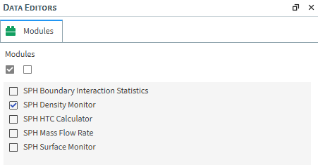
The embedded included by default in FreeFlow include the following:
SPH Boundary Interaction Statistics, which enables SPH boundary-related data, generating properties of the forces that the fluid is exerting on the walls. Also, curves may be generated for the resultant forces, torques and power.
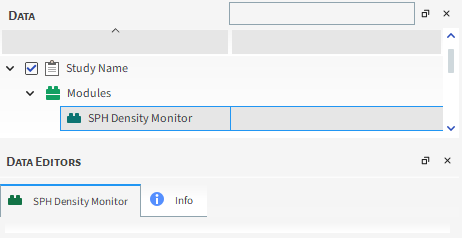
SPH Density Monitor, which enables the monitoring of density values of the SPH elements in a simulation.
SPH HTC Calculator, which calculates the heat transfer coefficient (HTC) through forced convection for each wall triangle.
SPH Mass Flow Rate, which enables the measurement of mass flow rate on the chosen surface.
SPH Surface Monitor, which
What would you like to do?
Learn about SPH Boundary Interaction Statistics Module
Learn about SPH Density Monitor Module
Learn about SPH HTC Calculator Module
Learn about SPH Mass Flow Rate Module
Learn about SPH Surface Monitor Module
SPH Boundary Interaction Statistics Module
The SPH Boundary Interaction Statistics Module enables a collection of SPH boundary-related data, separated into Boundary Properties, where SPH forces are divided into triangles and the nodal force is collected, and Boundary Curves where the collected value refers to the entire geometry.
Module Options
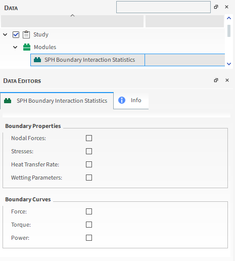
When the SPH Boundary Interaction Statistics Module is enabled (Figure 3.105: SPH Boundary Interaction Statistics Module Options), you are able to select any of the following parameters:
Boundary Properties
Nodal Forces
Stresses
The Stresses parameter calculates the time average of the stresses on the triangle. If there is no motion and the Cartesian forces are already stored, stresses are calculated with them, otherwise, normal and tangential components of the forces are stored.
Heat Transfer Rate
The Heat transfer rate parameter calculates the time average of the heat transferred between the fluid and the triangle (positive if the transfer is triangle->fluid, negative otherwise).
Wetting Parameters
The Wetting parameters calculates the time average of the ratio between the wet area (approximate) and the triangle area.
Note: Due the use of a kernel function for approximating the wet area, SPH elements located within a distance equal to the kernel radius from a boundary triangle will contribute to that area. This means that if a moving wall approaches an SPH free surface, for instance, it may show wet fractions above zero before actually touching the SPH elements.
Boundary Curves
Force;
Torque;
Power.
After processing your simulation, specific data based on the options you enabled will be available in Walls Properties or Curves. As you can see in the figures below:
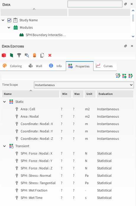
Walls-Properties
Figure 3.106: Results in Walls Properties when the SPH Boundary Interaction Statistics Module is Enabled
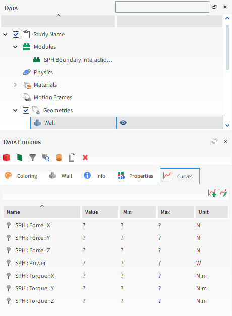
Walls-Curves
Figure 3.107: Results in Walls Curves when the SPH Boundary Interaction Statistics Module is Enabled
See also:
The SPH Density Monitor Module enables the monitoring of density values of the SPH elements during a simulation.
During the simulation, if the module detects that the density values were clipped due the existence of positive or negative deviations that exceeded the maximum allowed values, it will issue a warning, indicating the percentage of SPH elements that had density values clipped. These Warnings are registered in the log file and can be consulted later.
See the example in the figure below:

See also:
The SPH HTC Calculator module calculates the heat transfer coefficient (HTC) through forced convection for each wall triangle. It provides an estimation of heat exchange without requiring a thermal solution.
The heat transfer coefficient is calculated using simple correlations based on local Reynolds and Prandtl numbers. The correlations used for computing the Nusselt number depend on whether the flow is laminar or turbulent, as determined by the user-defined threshold.
Limitations
Listed below are known limitations of the SPH HTC Calculator module:
User input is required for fluid thermal conductivity and specific heat.
The module ignores the internal values of these properties in the fluid material. However, fluid viscosity is still extracted from the fluid material data.
The heat transfer coefficient is computed based on the local Nusselt number, which utilizes the fluid velocity at a specific distance from the wall, as determined by the Distance Factor.
You have the ability to modify the parameters utilized for calculating the Nusselt number in accordance with the flow characteristics.
Module Options
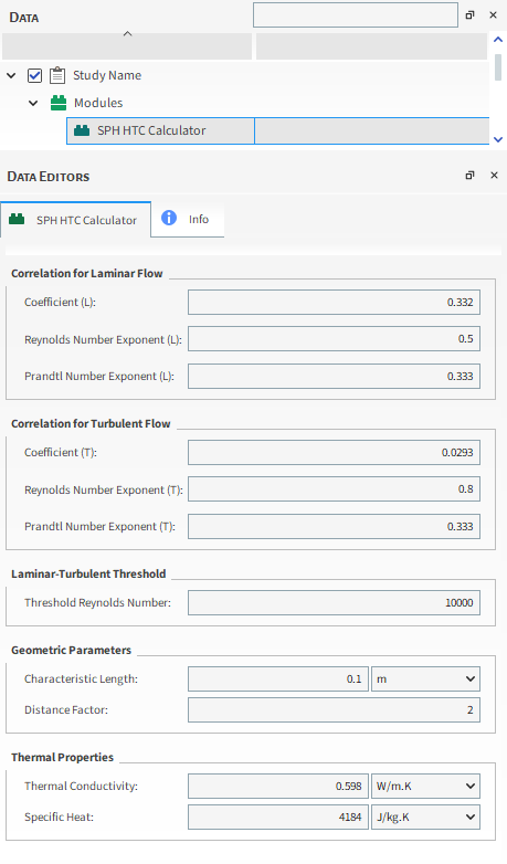
Refer to the Figure 3.111: Options in the Data Editors Panel when the SPH HTC Calculator is Enabled and the parameter definitions below to understand how to enable and configure the SPH HTC Calculator module.
Coefficient (L): Coefficient used to compute the Nusselt number for a laminar flow. Range: [Positive values]
Reynolds Number Exponent (L): Exponent that raises the Reynolds number to compute the Nusselt number for a laminar flow. Range: [Positive values]
Prandtl Number Exponent (L): Exponent that raises the Prandtl number to compute the Nusselt number for a laminar flow. Range: [Positive values]
Coefficient (T): Coefficient used to compute the Nusselt number for a turbulent flow. Range: [Positive values]
Reynolds Number Exponent (T): Exponent that raises the Reynolds number to compute the Nusselt number for a turbulent flow. Range: [Positive values]
Prandtl Number Exponent (T): Exponent that raises the Prandtl number to compute the Nusselt number for a turbulent flow. Range: [Positive values]
Threshold Reynolds Number: This defines the laminarturbulent transition. Above this Reynolds number, the flow is considered turbulent. Range: [Positive values]
Characteristic Length: Length used to compute the Reynolds number and the heat transfer coefficient. Range: [Positive values]
Distance Factor: Factor that multiplies the SPH element spacing for computing the distance from the wall at which the velocity is obtained. Range: [Positive values]
Thermal Conductivity: This defines the fluid thermal conductivity, which is used to compute the Prandtl number and the heat transfer coefficient. Range: [Positive values]
Specific Heat: This defines the specific heat used to compute the Prandtl number. Range: [Positive values]
Post-processing abilities
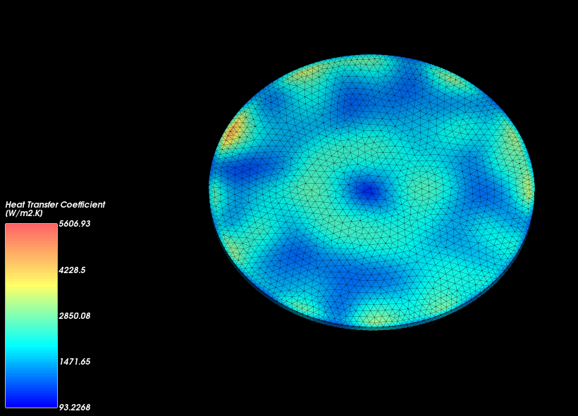
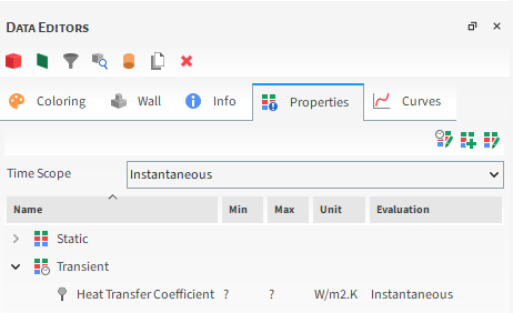
After simulating, a new Heat Transfer Coefficient property becomes available for wall entities, as shown in the figure below. This property aids in visualizing heat exchange between the SPH fluid and each wall.
Figure 3.112: New Property Shown in Data Editors Panel When the SPH HTC Calculator Module is Enabled
This property is explained below:
Heat Transfer Coefficient: This provides the heat transfer coefficient for each wall triangle.
You can analyze this property in a plot or histogram window. Alternatively, you can graphically display this property in a 3D View window.
Setting up and using the module
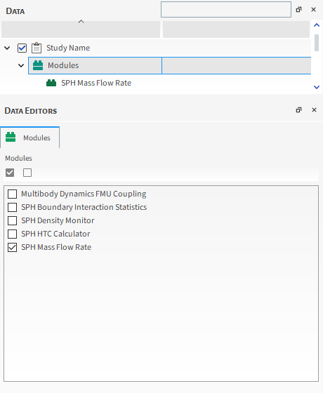
Ensure that the module is enabled. (From the Data panel, select Modules and then from the Data Editors panel, ensure the SPH HTC Calculator checkbox is enabled.)
From the Data panel, under Modules , select the new SPH HTC Calculator entry.
From the Data Editors panel, on the SPH HTC Calculator tab, enter the values you want.
Continue setting up the simulation as you normally would.
Process the simulation as you normally would.
When you are ready to post-process your simulation results, you can make use of the new parameter on the Properties tab for the main SPH entity.
See also:
The SPH Mass Flow Rate module is a flow meter that acts by calculating the SPH mass flow rate through a surface, enabling you to choose where you want to measure the mass flow rate.
Module Options
When the SPH Mass flow Rate Module is enabled (Figure 3.114: Geometries Options in the Data Editors Panel when the SPH Mass Flow Rate Module is Enabled), you are able to select one or more surfaces present in the simulation and measure the mass flow rate through them.
Figure 3.114: Geometries Options in the Data Editors Panel when the SPH Mass Flow Rate Module is Enabled
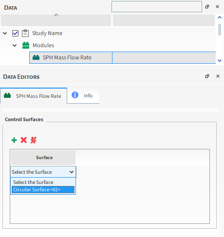
After processing your simulation, specific mass flow rate curves will be available for the surfaces you selected through the module.
See also:
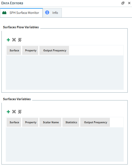
The SPH Surface Monitor module allows you to select one or more surfaces from the simulation and track SPH properties on those surfaces. Additionally, you can also define the output frequency at which results are provided. This allows you to obtain results at a higher rate than that of the simulation output frequency.
Module Options
When the SPH Surface Monitor Module is enabled, two fields become available:
Surfaces Flow Variables
Surfaces Variables
The Surfaces Flow Variables field allows you to choose between Mass and Count properties, both at Output frequency or Solver Curves frequency, for as many surfaces as necessary.
Meanwhile, aside from allowing you to select any simulation surface and define the desired output frequency, the Surfaces Variables field also enables a wider range of SPH Properties and the option to track a Scalar. Additionally, it allows you to select different Statistics to plot.
Note: The Scalar Name option enables you to analyze a property from another Module in your simulation.
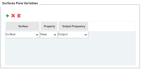
To use the Surfaces Flow Variables option, follow the steps below:
In the Surfaces Flow Variables field, click the Add button to create a new entry.
From the Surface dropdown list, select the simulation surface you want.
From the Property dropdown list, select one of the properties:
Mass
Count
From the Output Frequency dropdown list, select one of the options:
Output
Solver Curves
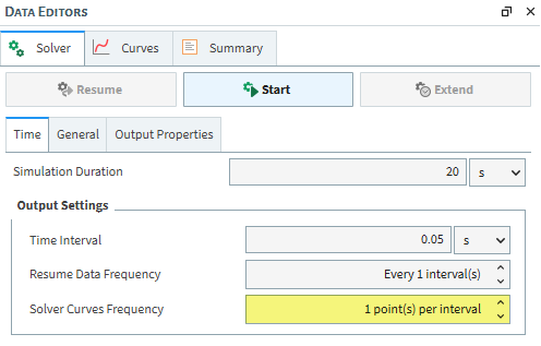
If you choose the Solver Curves option, there is an additional step to configure the desired frequency. Follow the points below:
From the Solver entity, navigate to the Time tab.
Under the Output Settings field, you will find the Solver Curves Frequency entry.
Here you will define how many times between Time Intervals the Solver will generate outputs for the selected property.
See below an example of the Surfaces Flow Variables setup:
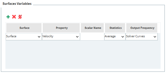
To use the Surfaces Variables option, follow the steps below:
From the Solver entity, navigate to the Time tab.
From the Surface dropdown list, select the simulation surface you want.
In this option, you have to either choose a Property or name a Scalar.
Important: Selecting a Property and naming a Scalar in the same entry will cause your simulation to break.
In case you need to analyze an SPH Property, you can choose between:
Count
Density
Mass
Pressure
Temperature
Velocity
Turbulent Viscosity
Molecular Viscosity
Volume
In case you need to track a Scalar, do the following:
This option works if you have another module enabled, and if said module enables a new property for the SPH entity. In this document, the SPH Air Drag Module will be used as an example. This module enables the Drag Force property.
In the Scalar Name field, type the name of the module's property. As an example, wishing to track the Drag Force provided by the SPH Air Drag Module, you would type "Drag Force".
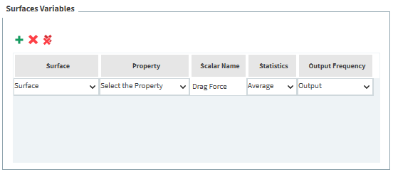
Next, from the Statistics dropdown list, select the statistic you wish:
Average
Minimum
Maximum
Sum
From the Output Frequency dropdown list, select one of the options:
Output
Solver Curves
If you choose the Solver Curves option, there is an additional step to configure the desired frequency. Follow the points below:
From the Solver entity, navigate to the Time tab.
Under the Output Settings field, you will find the Solver Curves Frequency entry.
Here you will define how many times between Time Intervals the Solver will generate outputs for the selected property.
See below an example of the Surfaces Variables setup:
Note: You can always create a new entry to cover all of the desired surfaces, properties and statistics.
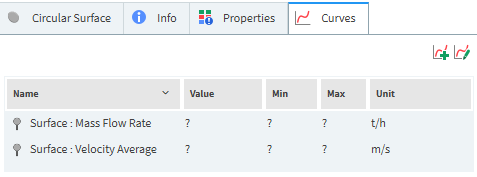
When the setup is finished, you can run the simulation.
After the simulation has been processed, the resulting curves will be available at the Curves tab of the surface or surfaces that you selected as entries in the SPH Surface Monitor Module.
Important:
You can make use of this module to track a certain simulation property until it reaches a steadystate, for example, so it will be up to you whether to continue or stop the simulation.
In some cases, there are only a few properties of interest, you can use this module to evaluate the desired properties and disable the collection of those that are not important in the context of your simulation, gaining processing speed and generating less data.
See also:
You may have access to other external Modules not included by default in Feeflow. These custom Modules might have been created by you using the FreeFlow Software Development Kit (SDK), separate functionality provided to you through the Ansys Learning Hub.
Tip: To learn more about making your own custom Modules:
Access the FreeFlow Solver SDK Manual. From the Help menu, point to Ansys FreeFlow Resources, and then click Solver SDK Manual.
External Modules are typically installed via ZIP file (see also Install an External Module). After installation, they will appear in FreeFlow under Modules in the Data panel.
Because these Modules are installed separately from the FreeFlow product, their documentation (if available) will be separate, too.
Tip: You will know if an external Module has included documentation if you see an Open this Module's Help File icon (?) on the Module's main tab in the Data Editors panel. Clicking this icon should open the Module's documentation in a separate window.
See also:
FreeFlow SIMULATION ENTITIES THAT CAN BE AFFECTED BY MODULES
Once you enable a Module (see also About Modules Parameters), there can be other places in the FreeFlow UI affected by that particular Module. How and which simulation entities can be affected depends upon the Module and how it was built.
What would you like to do?
Learn about Module Related Effects on the FreeFlow UI
Learn about Exclusive Settings
Learn about Non-Exclusive Settings
MODULE-RELATED EFFECTS ON THE FreeFlow UI
Typically, enabling a Module can affect the FreeFlow UI in one or more of the following ways:
The Module overrides FreeFlow's default models or settings. Models or settings that can be overwritten by a Module are considered to be exclusive. An exclusive model or setting allows a Module to disable its default options and replace them with the name of the Module.
The Module adds additional models or settings. Models or settings that are added to the FreeFlow UI as a result of enabling a Module are considered to be non-exclusive. A non-exclusive model or setting allows a Module to add new options to its default set of options, but does not allow the Module to override any default options.
See the below sections for more detail about each of these two Module-related UI conditions. In addition, refer to Table below to learn what areas of the FreeFlow UI might be affected by a Module.
FreeFlow UI settings that are considered to be exclusive have the effect of disabling FreeFlow's default options for a particular model or setting, and then replacing them with the name of the Module. In these cases, you must use the model or setting defined in the enabled Module, and only one enabled Module can override any particular model or setting at one time. This means that if you happen to have more than one Module defining the same exclusive model or setting in different ways, you must enable only one of those Modules in your simulation setup.
FreeFlow UI settings that are considered to be non-exclusive have the effect of adding in additional models or settings for the Module, but do not override any default models or settings. Sometimes the additional models or settings appear on a separate Modules tab within the affected simulation entity, and sometimes new options are added to existing entities or lists.
No matter how these appear to you in the UI, if you have enabled a Module that includes additional models or settings, you must make use of those Module-related models or settings at least once in your simulation setup.
SIMULATION ENTITIES THAT CAN BE AFFECTED BY MODULES
The table below lists the areas of the FreeFlow UI that are able to have their settings and options modified by a Module that is enabled.
Tip: Refer to the Module's documentation for further details about Module-specific parameters. Specifically:
For embedded Modules, this documentation can be found in the FreeFlow User Manual (the document you are reading now).
For external Modules, this documentation (if provided) can be found by clicking the Open this Module's Help File icon (?) on the Module's main tab in the Data Editors panel.
Table 1: Simulation Entities that can be affected by Modules, and how they can be affected
|
Simulation Entity |
Setting or Area Affected |
How Affected |
See Also |
|---|---|---|---|
|
Physics | Momentum tab |
Normal Force; Tangential Force; Adhesive Force; Impact Energy |
Built-in model override (exclusive settings) | |
|
Physics | Thermal tab |
Heat Conduction Model; Thermal Integration Model |
Built-in model override (exclusive settings) | |
|
Individual imported Geometries |
New Modules sub-tab |
Additional settings added | |
|
Individual Materials |
For each Material defined under Materials, a new group box labeled with the Module's name |
Additional settings added | |
|
Inlets and Outlets |
New Modules sub-tab |
Additional settings added |
What would you like to do?
In this version of FreeFlow, many more additional models and functionality are available as external Modules that can be downloaded from the Customer Portal.
Note: Even though this install procedure is similar on both Windows and Linux machines, be aware that Module ZIP files are specific to both the operating system and the version of FreeFlow for which the Module was created.
Locate or download the ZIP file for the external Module you want to install.
Into your user folder's
..FreeFlowModulesfolder, extract the contents of the ZIP file. For example:In Windows, this might be your
%USERPROFILE%/Documents/FreeFlow/Modulesfolder.In Linux, this might be your
~/.FreeFlow/Modulesfolder.
Once extracted, the ZIP file will automatically create a build folder in the
Modulesfolder and the Module contents will be installed there.If the FreeFlow program is open, close it and open it again to refresh the Modules list. The external Module should be listed in the Modules entity. (From the Data panel, select Modules and then from the Data Editors panel, review the Modules list.)
Tip: The available External Modules can be downloaded from the Customer Portal in the FreeFlow Section inside Add-On Packages.
Ensure that the ZIP file you download is appropriate for both the operating system and the FreeFlow version you are using.
See Also: