


The properties presented on the Properties and Curves tabs represent the many different statistics that FreeFlow records at each timestep for each individual element in a structure (e.g., SPH element, geometry triangle) as your simulation processes. The large amount of data that FreeFlow collects is then distilled into default properties that are accessible from either the Properties or Curves tab for the entity of interest.
Once a property is selected, you can quickly display individual statistics, visualize the data set in a 3D View, graph them in a plot or histogram, or export them in tabular format. You may also customize the default properties FreeFlow provides to create your own unique data sets, including limiting properties by a specific time range by using Time Statistics.
Note: The process for customizing default properties for Eulerian Statistics User Processes is slightly different from other entities (see also About Customizing Eulerian Statistics Properties.)
If you need to distill a data set from a property into one final value, or analyze the components that make up your data set, you can do so from the Output tab of the Expressions/Variables panel.
To help you choose the correct property, FreeFlow separates them into the following two categories:
Properties contain data sets that include recorded values for each individual element in a structure at each individual timestep during the simulation. This has the potential of producing many unique values per timestep.
Curves contain data sets that apply to the entire entity as a whole, producing only one value for each property.
What would you like to do?
See Also:
Properties are data sets that include recorded values for each individual element in a structure (e.g., SPH element, geometry triangle) at each individual output time during the simulation.
LIMITING AND DISPLAYING PROPERTIES
Because they have the potential to produce many unique values for each output time, Properties must first be limited by some factor (e.g., showing the data for only one output at a time, showing only the minimum or average value for all output times, and so on) before displaying it in the FreeFlow UI.
The ways in which you can limit and display your Properties are described in Table 1.
Table 1: Methods for Limiting What a Property will Display
|
Limit By |
Method |
See Also |
|---|---|---|
|
Operations | ||
|
By operations only |
Create a Time Plot from the property and then choose to limit the values by one of the operations provided, which include Min, Max, Sum, Sum Squared, Average, Variance, and Std. Deviation. | |
|
By both output time and operations |
From the property, choose to Compute Statistics for a single output time and then use the UI to display the individual values you want. The values you can display include the same operations used to limit a Time Plot (Min, Max, and so on) but also include Name, Unit, Type, and Location. | |
|
Output Time Only | ||
|
By creating a 3D View window |
Create a 3D View from the function and then use the Time toolbar to walk through the data collected for each individual output time (see also About the Time Toolbar). | |
|
By creating a Histogram |
Create a Histogram from the property and then use the Time toolbar to walk through the data collected for each individual output time (see also About the Time Toolbar). |
FreeFlow calculates Properties for individual geometry components, SPH, Eulerian Statistics and individual User Processes based upon these entities.
Note: When displaying Properties for a User Process, the properties displayed will be those belonging to the linked entity upon which the User Process was based.
If these default properties do not meet your needs, you may also create custom Properties (see also About Customizing Properties or Curves), including Time Statistics Properties, which limits properties by a time range (see also About Adding and Editing Time Statistics Properties).
A list of available properties appears for each applicable component after processing via the component's Properties tab. Next to each property name row are various columns representing specific categories of operations and other data.
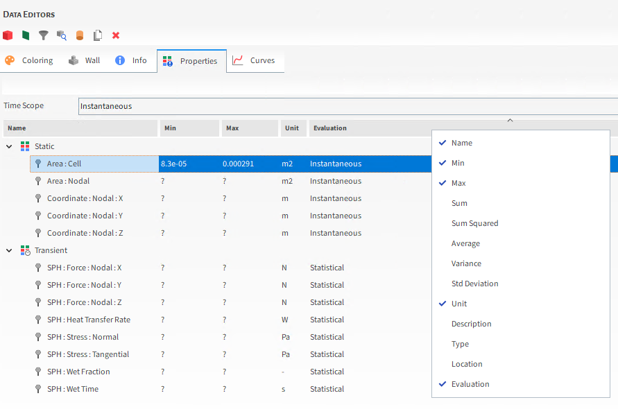
Besides separate columns for all standard operators—which include values for Min, Max, Sum, Sum Squared, Average, Variance, and Std. Deviation, that you can access by right-clicking the main bar—you can also view the property's Units, Type, Location, and Evaluation.
By right-clicking a property row and then selecting Compute statistics, you can get values for that property at that particular output (see also About Viewing an Individual Statistic).
DEFINITIONS OF DEFAULT FREEFLOW PROPERTIES
See the images and tables below to learn about the various Properties available by default in FreeFlow.
TIME SCOPE FOR PROPERTIES
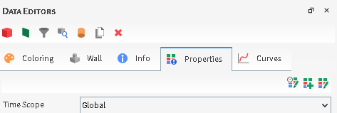
Table 2: Properties available by default for all entities
|
Property Name |
Description |
|---|---|
|
Time Scope |
Sets how the resulting statistics are displayed in the various factor columns. Specifically:
|
GEOMETRY COMPONENT PROPERTIES
There are two kinds of Properties for individual Geometry components:
Standard properties, which are calculated by default for every imported Geometry.
Collision statistics properties, which are collected only when the SPH Boundary Interaction Statistics collection feature is enabled.
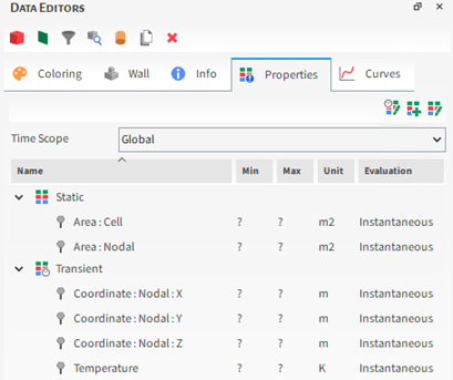
Figure 5.4: SPH Boundary Interaction Statistics Properties on the Data Editors panel for Geometry components
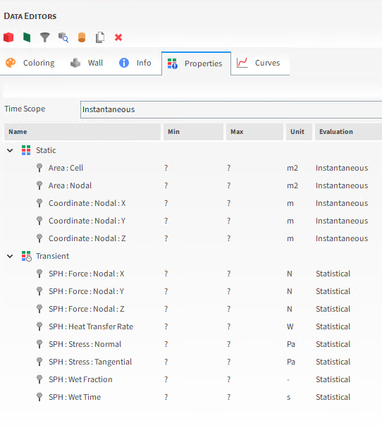
Table 3: Properties available by default for Geometries.
|
Property Name |
Description |
|---|---|
|
Standard Properties | |
|
Area : Cell |
The surface area of each individual triangle that makes up the selected geometry. |
|
Area : Nodal |
The area of a region around each individual geometry node. This area is equal to the sum of one third of the area of all triangles that share a given node. |
|
Coordinate : Nodal : X |
The coordinate location along the X axis for each individual geometry node. |
|
Coordinate : Nodal : Y |
The coordinate location along the Y axis for each individual geometry node. |
|
Coordinate : Nodal : Z |
The coordinate location along the Z axis for each individual geometry node. |
|
Temperature |
When Thermal Model is enabled, this is the thermodynamic temperature of each individual triangle that makes up the selected geometry. |
|
SPH Boundary Interaction Statistics Properties | |
|
SPH : Force : Nodal : X |
When the Nodal Forces option is enabled on the SPH Boundary Interaction Statistics module, this provides the average force in the X direction for each individual geometry node. |
|
SPH : Force : Nodal : Y |
When the Nodal Forces option is enabled on the SPH Boundary Interaction Statistics module, this provides the average force in the Y direction for each individual geometry node. |
|
SPH : Force : Nodal : Z |
When the Nodal Forces option is enabled on the SPH Boundary Interaction Statistics module, this provides the average force in the Z direction for each individual geometry node. |
| SPH : Stress : Normal |
When the Stresses option is enabled on the SPH Boundary Interaction Statistics module, this provides the average stress in the normal direction for each individual geometry triangle. |
| SPH : Stress : Tangential |
When the Stresses option is enabled on the SPH Boundary Interaction Statistics module, this provides the average stress in the tangential direction for each individual geometry triangle. |
| SPH : Wet Fraction |
When the Wetting Parameters option is enabled on the SPH Boundary Interaction Statistics module, this provides the wet fraction for each individual geometry triangle. In other words, it is the time average of the ratio between the approximate wet area and the triangle area |
| SPH : Wet Time |
When the Wetting Parameters option is enabled on the SPH Boundary Interaction Statistics module, this provides the time that a triangle was wet during the lapse between two consecutive outputs. For a boundary triangle to be considered wet at a given time, at least one SPH element must be interacting with the triangle. |
Tip: See the FreeFlow SPH Technical Manual available on the FreeFlow Help page for more information about the presented SPH properties.
SPH PROPERTIES
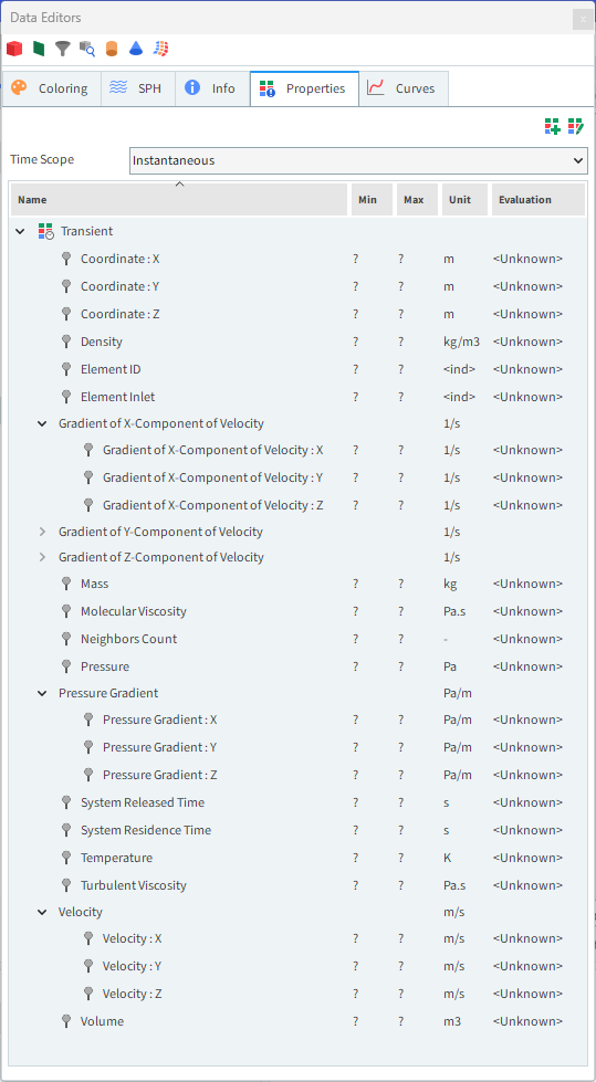
Table 7: Properties available when running a SPH simulation
|
Property Name |
Description |
|---|---|
|
Coordinate : X |
The Coordinate component in the X direction for each SPH element. |
|
Coordinate : Y |
The Coordinate component in the Y direction for each SPH element. |
|
Coordinate : Z |
The Coordinate component in the Z direction for each SPH element. |
|
Density |
The density of each SPH element |
|
Element ID |
The numeric identifier unique to each individual SPH element. |
| Element Inlet |
The name of the inlet through which each individual SPH element originally entered the simulation. |
| Gradient of X-Component of Velocity : X | The X-direction gradient of the X-component of Velocity. |
| Gradient of X-Component of Velocity : Y | The Y-direction gradient of the X-component of Velocity. |
| Gradient of X-Component of Velocity : Z | The Z-direction gradient of the X-component of Velocity. |
| Gradient of Y-Component of Velocity : X | The X-direction gradient of the Y-component of Velocity. |
| Gradient of Y-Component of Velocity : Y | The Y-direction gradient of the Y-component of Velocity. |
| Gradient of Y-Component of Velocity : Z | The Z-direction gradient of the Y-component of Velocity. |
| Gradient of Z-Component of Velocity : X | The X-direction gradient of the Z-component of Velocity. |
| Gradient of Z-Component of Velocity : Y | The Y-direction gradient of the Z-component of Velocity. |
| Gradient of Z-Component of Velocity : Z | The Z-direction gradient of the Z-component of Velocity. |
| Mass | The mass of each individual SPH element. |
| Molecular Viscosity | The viscosity associated to each SPH element. |
|
Neighbors Count |
Count of neighbor SPH elements. |
|
Pressure |
The pressure that each SPH element is subjected to. |
| Pressure Gradient : X | The pressure gradient in the X-direction. |
| Pressure Gradient : Y | The pressure gradient in the Y-direction. |
| Pressure Gradient : Z | The pressure gradient in the Z-direction. |
| Refinement Count | Indicates the level of refinement of the SPH elements. The range is
from 1, which is the most refined SPH element and the maximum value is
 , where n is the biggest Level of Refinement
set in the Adaptive Sizing tab. , where n is the biggest Level of Refinement
set in the Adaptive Sizing tab. |
| System Released Time |
The instance in simulation time when each individual SPH element originally entered the simulation domain. |
| System Residence Time | The amount of time each individual SPH element has been within the simulation
domains. It can be defined as the difference between the current time,
 , and the time the SPH element entered the simulation, , and the time the SPH element entered the simulation,
 . .Therefore, |
|
Temperature |
Temperature of SPH elements. |
|
Turbulent Viscosity |
The turbulent viscosity associated to each SPH element. Note: This property is only available if a turbulence model is enabled. |
|
Velocity : X |
The velocity vector component in the X direction for each SPH element. |
|
Velocity : Y |
The velocity vector component in the Y direction for each SPH element. |
|
Velocity : Z |
The velocity vector component in the Z direction for each SPH element. |
| Volume | The volume of each individual SPH element. |

EULERIAN STATISTICS PROPERTIES
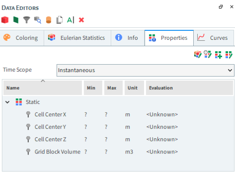
Table 11: Properties available by default for Eulerian Statistics
|
Property Name |
Description |
|---|---|
| Cell Center X |
Eulerian bin coordinates in the X direction. Useful for analyzing properties that can vary spatially, you can create a Cross Plot of a certain property over the bin coordinates in the X direction. |
| Cell Center Y |
Eulerian bin coordinates in the Y direction. Useful for analyzing properties that can vary spatially, you can create a Cross Plot of a certain property over the bin coordinates in the Y direction. |
| Cell Center Z |
Eulerian bin coordinates in the Z direction. Useful for analyzing properties that can vary spatially, you can create a Cross Plot of a certain property over the bin coordinates in the Z direction. |
|
Grid Block Volume |
The total volume of each individual block the Cube or Cylinder User Process is divided into (see also About Eulerian Statistics). |
What would you like to do?
See Also:
Unlike Properties, which record many individual values for each output time, the Curves tab displays only the entity properties that produce a single value. This means that a Property becomes a Curve after its data set is reduced to a single value; for example, by choosing to sum all the values or average them out.
Curves are calculated using Global coordinates and are collected for geometry components, as well as for the Solver and individual Motion Frames. And as with Properties, individual User Processes linked to any entities with Curve properties will also display the same properties on their own Curves tabs.
Unlike Properties, you cannot display Curves in a 3D View or a Histogram due to the one-dimensional aspect of the data that is recorded. The ways in which you can display Curves in the FreeFlow UI are described in the table below.
Table 1: Methods for Displaying Curves data
|
Display Options |
Method |
See Also |
|---|---|---|
|
Through the Curves tab |
From the property, choose to Compute Statistics and then use the UI to display the individual values you want. | |
|
In a Time Plot |
Create a Time Plot from the property. |
ABOUT CURVES FOR IMPORTED GEOMETRIES AND MOTION FRAMES
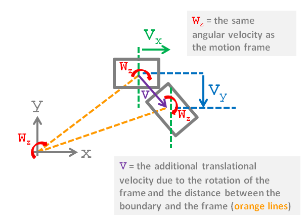
In FreeFlow, both imported Geometries and Motion Frames have Curves properties available, both of which provide translational and angular velocities in different directions. At first glance, it might appear that the velocity values for an imported geometry might be equal to those of the Motion Frame assigned to it, but this is not always the case, as described below and illustrated in Figure 5.7: Diagram showing how Motion Frames assigned to a rectangular boundary affect the resulting velocity Curves for the boundary
In cases where the Motion Frame assigned to the geometry has only translation motions, the boundary velocities will be equal to that of the Motion Frame.
In cases where the Motion Frame assigned to the geometry has only rotation motions, the boundary will have the same angular velocity as the Motion Frame plus a separate translational velocity as given by the angular velocity of the frame and the distance between the boundary and the frame (see Figure 1).
In cases where the Motion Frame assigned to the geometry has both translation and rotation motions, the boundary will have the same angular velocity and a combination of the frame's translational velocity and the additional translational velocity applied due to the frame's rotation and the distance between the boundary and the frame.
Figure 5.7: Diagram showing how Motion Frames assigned to a rectangular boundary affect the resulting velocity Curves for the boundary
DEFINITIONS OF FREEFLOW CURVES
See the images and tables below to learn about the various Curves available in FreeFlow.
GEOMETRY COMPONENT CURVES
Figure 5.8: Geometry Curves options on the Data Editors panel when SPH Boundary Interaction Statistics are collected
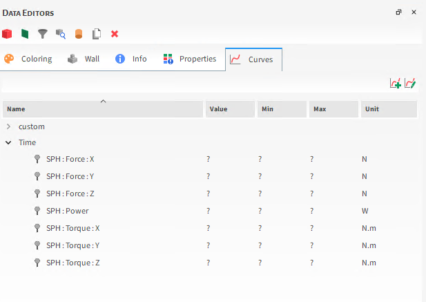
Figure 5.9: Imported wall Geometry, Curves options on the Data Editors panel when Motion Frames are assigned
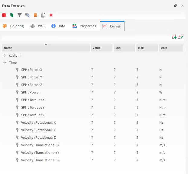
Table 2: Curves options for Geometries
|
Function |
Description |
|---|---|
|
Geometries When SPH Boundary Interaction Statistics are collected. | |
|
SPH : Force : X |
When the Force option is enabled on the SPH Boundary Interaction Statistics module, this provides the force applied to the geometry along the X axis. |
|
SPH : Force : Y |
When the Force option is enabled on the SPH Boundary Interaction Statistics module, this provides the force applied to the geometry along the Y axis. |
|
SPH : Force : Z |
When the Force option is enabled on the SPH Boundary Interaction Statistics module, this provides the force applied to the geometry along the Z axis. |
|
SPH : Power |
When the Power option is enabled on the SPH Boundary Interaction Statistics module, this provides the power required to move the geometry at the specified speed given the fluid load applied to the surface. This is useful for determining the power applied by the geometry. |
| SPH : Torque : X | When the Torque option is enabled on the SPH Boundary Interaction Statistics module, this provides the torque required to rotate the geometry around the X axis at the specified speed given the fluid load applied to the surface. |
| SPH : Torque : Y | When the Torque option is enabled on the SPH Boundary Interaction Statistics module, this provides the torque required to rotate the geometry around the Y axis at the specified speed given the fluid load applied to the surface. |
| SPH : Torque : Z | When the Torque option is enabled on the SPH Boundary Interaction Statistics module, this provides the torque required to rotate the geometry around the Z axis at the specified speed given the fluid load applied to the surface. |
|
Geometries When Motion Frames are assigned | |
|
Velocity : Rotational : X |
When the geometry has a Motion Frame assigned to it, this is the rotational (angular) velocity of the assigned Motion Frame as defined in the X direction. |
|
Velocity : Rotational : Y |
When the geometry has a Motion Frame assigned to it, this is the rotational (angular) velocity of the assigned Motion Frame as defined in the Y direction. |
|
Velocity : Rotational : Z |
When the geometry has a Motion Frame assigned to it, this is the rotational (angular) velocity of the assigned Motion Frame as defined in the Z direction. |
|
Velocity : Translational : X |
When the geometry has a Motion Frame assigned to it, this is the translational velocity of the assigned Motion Frame as defined in the X direction. |
|
Velocity : Translational : Y |
When the geometry has a Motion Frame assigned to it, this is the translational velocity of the assigned Motion Frame as defined in the Y direction. |
|
Velocity : Translational : Z |
When the geometry has a Motion Frame assigned to it, this is the translational velocity of the assigned Motion Frame as defined in the Z direction. |
SOLVER CURVES
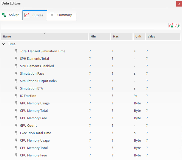
Table 7: Curves options for the Solver entity
|
Function |
Description |
|---|---|
|
CPU Memory Free |
The amount of memory available on the CPU. |
|
CPU Memory Total |
The total amount of memory—both used and unused—the CPU has. |
|
CPU Memory Usage |
The amount of memory that is being used on the CPU. |
|
Enabled SPH Elements |
The total number of SPH Elements that are currently located within the simulation boundaries. |
|
Execution Total Time |
The amount of time (duration) that has passed since the simulation started processing again from a stopped state. |
|
GPU Count |
The total number of GPU cards that are processing the simulation. |
|
GPU Memory Free |
The amount of memory available on the GPU(s) that is processing the simulation. |
|
GPU Memory Total |
The total amount of memory—both used and unused—that the GPU(s) processing the simulation has. |
|
GPU Memory Usage |
The amount of memory being used on the GPU(s) processing the simulation. |
|
Halo SPH Elements |
In multi-GPU runs, Halo SPH Elements are those that are located in the overlapping devices domain regions and therefore are present simultaneously in two GPU devices. For the Halo SPH Elements, both devices compute the collision forces but only one of the devices accumulates these data in order to perform velocity and displacement calculations. |
|
IO Fraction |
The fraction of each unit of simulation time allotted to I/O (input/output), which involves writing to and reading from the simulation information on disk. This fraction is a value between 0.0 and 1.0: when closer to 0.0, less wall clock time was spent on I/O. |
|
Simulation ETA |
The estimated amount of time (duration) required to finish processing the simulation. This value considers the current simulation configuration. |
|
Simulation Output Index |
The output file saved for the output time. This is useful for determining at what point during the simulation an event of interest occurred. |
|
Simulation Pace |
The estimated amount of time (duration) required to advance the simulation one second. This value considers the current simulation configuration. |
|
Halo SPH Elements Ratio |
The ratio between the number of halo elements and the total number of SPH Elements in the domain. |
|
Total Elapsed Simulation Time |
The total amount of time (duration) that the simulation has been processing since it was originally started. This is calculated by adding up the various Execution Total Times from multiple, separate executions (stops and resumes) of the simulation. |
MOTION FRAMES CURVES
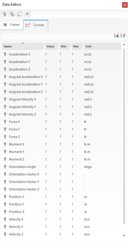
Table 8: Curves options for Motion Frames
|
Function |
Description |
|---|---|
|
Acceleration X |
The motion frame's acceleration along the X axis. |
|
Acceleration Y |
The motion frame's acceleration along the Y axis. |
|
Acceleration Z |
The motion frame's acceleration along the Z axis. |
|
Angular Acceleration X |
The X-component of the motion frame's angular acceleration vector. |
|
Angular Acceleration Y |
The Y-component of the motion frame's angular acceleration vector. |
|
Angular Acceleration Z |
The Z-component of the motion frame's angular acceleration vector. |
|
Angular Velocity X |
The X-component of the motion frame's angular velocity vector. |
|
Angular Velocity Y |
The Y-component of the motion frame's angular velocity vector. |
|
Angular Velocity Z |
The Z-component of the motion frame's angular velocity vector. |
|
Force X |
The force applied to the motion frame along the X axis. |
|
Force Y |
The force applied to the motion frame along the Y axis. |
|
Force Z |
The force applied to the motion frame along the Z axis. |
|
Moment X |
The moment (torque) applied to the motion frame along the X axis. |
|
Moment Y |
The moment (torque) applied to the motion frame along the Y axis. |
|
Moment Z |
The moment (torque) applied to the motion frame along the Z axis. |
|
Orientation Angle |
For the set of axes that represents the Motion Frame's orientation, this is the rotation angle about the defined Relative Rotation Vector. |
|
Orientation Vector X |
The X-component defining the vector about which the motion frame axes is rotated. |
|
Orientation Vector Y |
The Y-component defining the vector about which the motion frame axes is rotated. |
|
Orientation Vector Z |
The Z-component defining the vector about which the motion frame axes is rotated. |
|
Position X |
The coordinate location of the motion frame axes' center point as specified in the X direction. |
|
Position Y |
The coordinate location of the motion frame axes' center point as specified in the Y direction. |
|
Position Z |
The coordinate location of the motion frame axes' center point as specified in the Z direction. |
|
Velocity X |
The translational velocity of the motion frame as defined in the X direction. |
|
Velocity Y |
The translational velocity of the motion frame as defined in the Y direction. |
|
Velocity Z |
The translational velocity of the motion frame as defined in the Z direction. |
What would you like to do?
See Also:
There are many default properties provided on the Properties and Curves tabs for a simulation entity (SPH, Solver, individual geometry components, individual Motion Frames, Eulerian Statistics, and any individual User Processes linked to these entities) but you can also create and edit custom properties to create your own unique data sets.
Note: Though customizing Properties also applies to Eulerian Statistics, because Eulerian Statistics is a unique User Process based only upon the SPH entity, you can also add new SPH Properties to a Eulerian Statistics User Process. See About Customizing Eulerian Statistics Properties for more information.
Customizing Properties is accomplished from the upper-right corner of the Properties tab. Customizing Curves is accomplished from the upper-right corner of the Curves tab.
CUSTOM PROPERTIES OR CURVES PARAMETER DEFINITIONS
See the images and tables below to help you understand how to add and edit your own unique properties or curves.
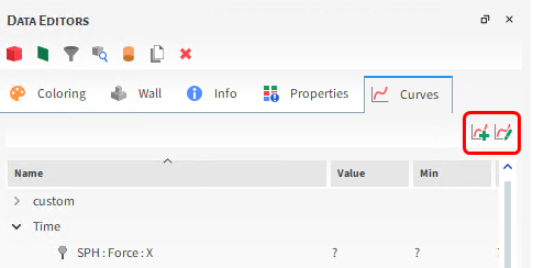
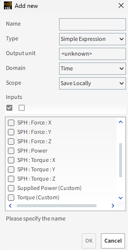
Table 1 : Add new dialog options (property or curve)
|
Setting |
Description |
Range |
|---|---|---|
|
Name |
Enables you to specify a unique identifier for the property or curve. |
99 character limit |
|
Type |
Specifies how the expression will be defined.
Note: The expression is entered on the Custom Property or Custom Curves dialog that appears after you click OK (see below section.) |
Simple Expression; Advanced Expression (script) |
|
Output unit |
The units you want assigned to the property or curve. |
<unknown>; any applicable unit defined in FreeFlow . |
| Domain | The domain of the new Custom Property/Curve. | Time |
| Scope | Allows you to save the Property or Curve in your local desktop or only in the project. | Save Locally, Save in Project |
|
Inputs |
Lists all existing properties or curves available for the entity, including any custom properties or curves you have defined. |
Automatically provided. |
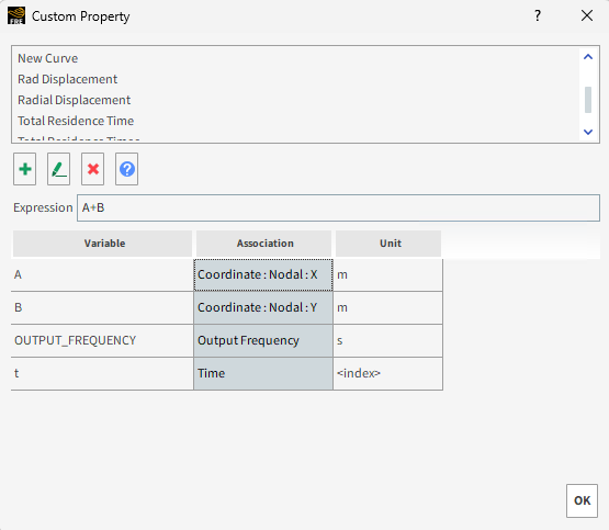
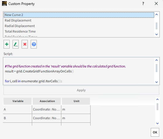
Table 2: Custom dialog options (properties and curves)
|
Setting |
Description |
Range |
|---|---|---|
|
Expression |
When the Type of the custom property or curve is Simple Expression, this is where you define the mathematical expression for the property or curve. | |
|
Script |
When the Type of the custom property or curve is Advanced Expression (script), this is where you use Python code to define the details of the property or curve. Note: The code you enter here is not the same as a FreeFlow script which has a different structure and purpose. | |
|
Variable |
Column that lists the variable names available for you to use within the expression or script. Specifically:
The following variables are also in the product but are not recommended for use at this time:
|
Automatically provided |
|
Association |
Column that maps the Variable name to its FreeFlow property. |
Automatically provided |
|
Unit |
Column that lists the unit used by the Variable. |
Automatically provided |
What would you like to do?
See Also:
You can customize Eulerian Statistics Properties just like any other Property (see also About Customizing Properties or Curves.) However, unlike other Properties, you may also add new SPH Properties to your default list of Eulerian Statistics Properties.
Eulerian Statistics is a unique User Process based only upon the SPH entity (see also About Eulerian Statistics). The primary purpose is to analyze specific locations in a simulation, and not necessarily the individual SPH elements that are in them. For example, you might use Eulerian Statistics to analyze the average SPH mass inside each individual block to see at a glance which region of your simulation has a higher density of SPH. So while the analysis uses information about the SPH, it is really the individual blocks and the simulation locations they represent that are the primary focus.
Thus, unlike other User Processes, which offer default Properties shared by the simulation entity upon which they were created, Eulerian Statistics has its own set of unique Properties (see also About Properties.) To these default functions, you can add additional Properties from the SPH entity upon which the Eulerian Statistics User Process is based.
See the images and table below to understand how to add SPH Properties to your Eulerian Statistics User Process.
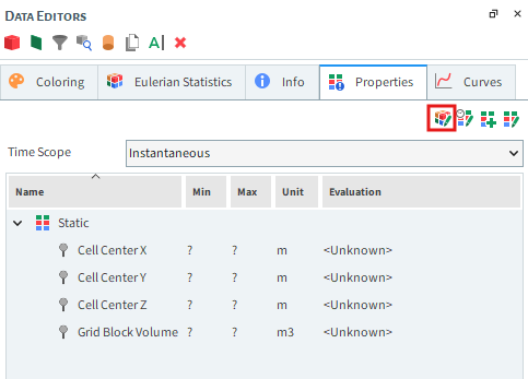
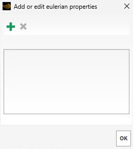
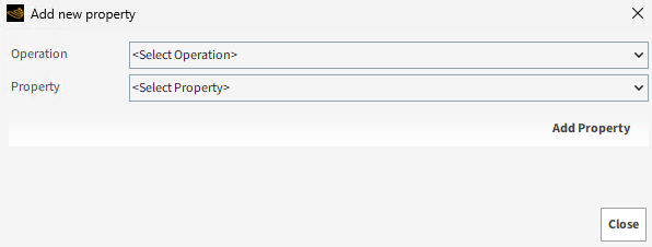
Table 1 : Add new property dialog options
|
Setting |
Description |
Range |
|---|---|---|
|
Operation |
The operation that will be applied to the SPH Property(s) selected. Specifically:
|
Average; Min; Max; Sum; Volume Fraction Average; Weighted Average; Standard Deviation |
|
Property |
Lists all existing properties available for the SPH entity, including any custom properties you have defined. |
Automatically provided. |
|
Weight Property |
When Weighted Average is chosen from the Operation list, this lists all existing properties available for the SPH entity, including any custom properties you have defined. |
Automatically provided. |


What would you like to do?
See Also:
You can customize the SPH Eulerian Solution Properties just like any other Property (see also About Customizing Properties or Curves.)
Eulerian Solution allows you to analyze specific locations in a simulation where there are no SPH elements in a specific time step. For example, you might use Eulerian Statistics to analyze the average density of each individual cell see at a glance which region of your simulation has a higher fluid density. So while the analysis uses information about the SPH elements, it is really the individual cells and the simulation locations they represent that are the primary focus.
The Eulerian Solution option has its own set of unique Properties (see also About Properties.) To these default functions, you can add additional Custom Properties.
See the image and table below to understand what Properties are available when using the Eulerian Solution.
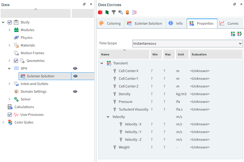
Table 1 : Properties available in the SPH Eulerian Solution
Property Name | Description |
|---|---|
| Cell Center X |
Eulerian bin coordinates in the X direction. Useful for analyzing properties that can vary spatially, you can create a Cross Plot of a certain property over the bin coordinates in the X direction. |
| Cell Center Y |
Eulerian bin coordinates in the Y direction. Useful for analyzing properties that can vary spatially, you can create a Cross Plot of a certain property over the bin coordinates in the Y direction. |
| Cell Center Z |
Eulerian bin coordinates in the Z direction. Useful for analyzing properties that can vary spatially, you can create a Cross Plot of a certain property over the bin coordinates in the Z direction. |
Density | The average density of each Eulerian Solution cell |
Pressure | The average pressure of each Eulerian Solution cell |
Turbulent Viscosity (only available if a turbulence model is enabled) | The average turbulent viscosity of each Eulerian Solution cell |
Velocity: X | The average X direction velocity of each Eulerian Solution cell |
Velocity: Y | The average Y direction velocity of each Eulerian Solution cell |
Velocity: Z | The average Z direction velocity of each Eulerian Solution cell |
Weight | Property that indicates from 0 to 1 how much fluid is present in a cell (0 no fluid, 1 full of fluid) |
See Also:
A Time Statistics Property enables you to limit a Property by a particular time range and operation that you specify. That new property definition becomes its own unique Property, which you can then use just like any other Property for further analysis. This method is useful when you need to focus your analysis upon only the average (max, min, or sum) values for a Property calculated during a certain time period of your simulation.
APPLYING TIME STATISTICS PROPERTIES
Time statistics are available for all Properties (see also About Properties) except those accessible via the main SPH entity. This includes support for all of the following entities:
Eulerian Statistics User Process Properties (see also About Eulerian Statistics.)
Individual Geometry component Properties.
Once you add a Time Statistics Property for one of the above supported entities, it will be available for all entities of the same type.
TIME STATISTICS PROPERTIES AND EULERIAN STATISTICS
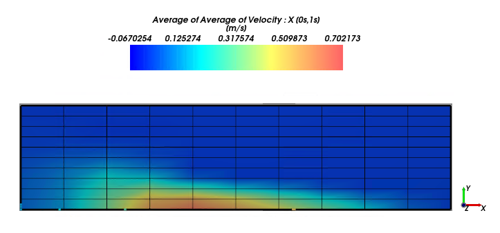
With regular Properties, the results by default only take into account data calculated for the current timestep (Figure 5.20: Water (SPH elements) colliding with column). By using by Eulerian Statistics User Process, for example, and then customizing the Properties (see also About Customizing Eulerian Statistics Properties), you could also show an operation (average, for example) for that same Property within the individual Eulerian blocks, but still for only one timestep at a time (Figure 5.22: The same setup and timestep as Figure 2, but showing with Eulerian Statistics applied, showing the average values of Velocity : X in each eulerian box (Eulerian Property)). With Time Statistics Properties, you can now apply an operation over a specific time range (Figure 5.23: The same mill and Eulerian Statistics applied as above, but now those values are averaged over a set range of time (Time Statistics Property from Velocity : X)).
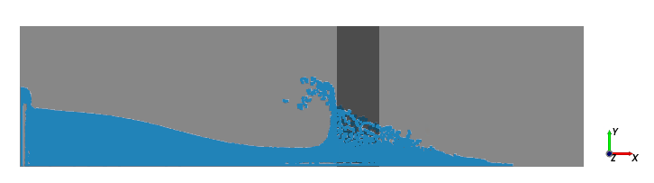
Figure 5.21: The same setup and timestep as above, but showing one Property, Velocity : X (standard Property)
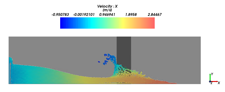
Figure 5.22: The same setup and timestep as Figure 2, but showing with Eulerian Statistics applied, showing the average values of Velocity : X in each eulerian box (Eulerian Property)
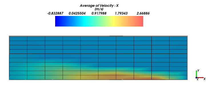
Figure 5.23: The same mill and Eulerian Statistics applied as above, but now those values are averaged over a set range of time (Time Statistics Property from Velocity : X)
TIME STATISTICS PROPERTIES PARAMETER DEFINITIONS
Like Customizing a Property (see About Customizing Properties or Curves), adding and editing Time Statistics Properties is accomplished from the upper-right corner of the Properties tab. See the images and tables below to help you understand how to add and edit Time Statistics Properties.
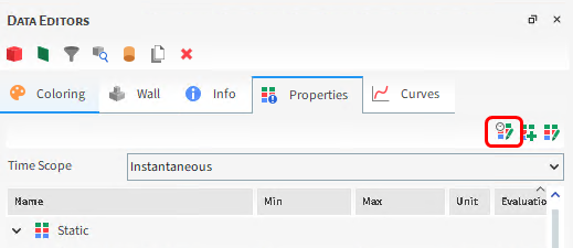
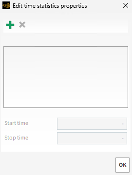
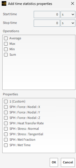
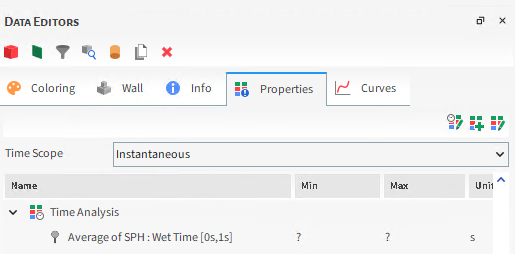
Table 1: Edit time statistics property dialog options
|
Setting |
Description |
Range |
|---|---|---|
|
Start Time |
The amount of time into your simulation that you want calculations to start being included in the operation selected for the Time Statistics Property. Note: Neither Time values are editable until you add a Time Statistics Property. To accomplish this, click the Add button. |
Positive values |
|
Stop Time |
The amount of time into your simulation that you want calculations to stop being included in the operation selected for the Time Statistics Property. Tip: If you want your range to extend to the end of your simulation, enter a very large number, such as 1000. Note: Neither Time values are editable until you add a Time Statistics Property. To accomplish this, click the Add button. |
Positive values |
Table 2: Add time statistics property dialog options
|
Setting |
Description |
Range |
|---|---|---|
|
Start Time |
The amount of time into your simulation that you want calculations to start being included in the operation selected for the Time Statistics Property. Between this and the Stop Time value defines the time range for the new Time Statistics Property. |
Positive values |
|
Stop Time |
The amount of time into your simulation that you want calculations to stop being included in the operation selected for the Time Statistics Property. Between the Start Time and this value defines the time range for the new Time Statistics Property. Tip: If you want your range to extend to the end of your simulation, enter a very large number, such as 1000. |
Positive values |
|
Operations |
Enables you to choose one or more operations to apply to the Property data within the time range you selected. One unique Time Statistics Property will be created per Operation and Property selected. Specifically:
|
Average; Min; Max; Sum |
|
Property |
Enables you to choose one or more Properties to which you can apply the selected Operations over the time range you selected. One unique Time Statistics Property with the selected time range will be created per Property and Operation selected. |
List provided automatically |


What would you like to do?`
See Also:
Note: This particular process does not apply to any SPH Properties added to a Eulerian Statistics User Process. See About Customizing Eulerian Statistics Properties for more information.
From the Data panel, select the entity containing the property you want to change or remove. This can include imported Geometries, SPH, Solver, or individual Motion Frame.
From the Data Editors panel, select either the Properties or Curves tab containing the custom property you want to change or remove.
From the upper right corner of the tab, click the Edit custom… button.
From the Custom… dialog, select the name of the property you want under Select Element.
Do any or all of the following:
To change the Name, Output unit, or Inputs used by the property, click the Edit…. button.
To change the expression listed in either the Expression or Script boxes, make your changes directly within the dialog.
To remove the function, click the Remove custom… button.
Click OK.
See Also:
Note: This particular process does not apply to any SPH Properties added to a Eulerian Statistics User Process. See About Customizing Eulerian Statistics Properties for more information.
From the Data panel, select the entity to which you want to add a custom property. This can include imported Geometries, SPH, Solver, individual Motion Frame, or any individual User Process linked to these entities.
From the Data Editors panel, select one of the following:
The Properties tab, to create a custom function applying to each individual element in a structure.
The Curves tab, to create a custom property applying to the entire entity as a whole.
From the upper right corner of the tab, click the Add new custom… button.
From the Add new dialog, enter the information you want, and then click OK. Tips: To select all inputs, click the Check All button. To clear all inputs, click the Uncheck All button.
From the Custom… dialog, define your expression in either the Expression or Script box shown using the variables provided in the dialog's table.
Click OK. The new custom property appears in the functions list sorted by Name.
See Also:
From the Data panel, under User Processes, select the Eulerian Statistics User Process you want (see also Divide a Cube or Cylinder User Process into Many Analysis Blocks.)
From the Data Editors panel, select the Properties tab.
From the upper-right corner of the tab, click the Add and edit properties for source entity button.
From the Add or edit eulerian properties dialog, click the Add button.
From the Add new property dialog, select the options you want, and then click Add Property. The new function appears on the Properties tab.
Repeat step 5 for each new function you want to add.
Click Close. The function(s) you added appear in the Add or edit eulerian properties dialog.
Click OK.
See Also:
Note: This procedure applies only to SPH Properties that you have added to a Eulerian Statistics User Process (see also Add a SPH Property to a Eulerian Statistics User Process.) You may not remove the SPH Properties provided by default with FreeFlow.
From the Data panel, under User Processes, select the Eulerian Statistics User Process containing the SPH Property you want to remove.
From the Data Editors panel, select the Properties tab.
From the upper-right corner of the tab, click the Add and edit properties for source entity button.
From the Add or edit eulerian properties dialog, select the SPH Property you want from the list, and then click the Remove button.
Click OK to close the dialog. Your changes are reflected in the Properties list for the Eulerian Statistic User Process.
See Also:
Note: This particular process does not apply to the main SPH entity, nor any User Process created from it, with the exception of Eulerian Statistics (see also About Eulerian Statistics.)
From the Data panel, select the entity to which you want to add a Time Statistics Property. This can include imported Geometries, Eulerian Statistics User Process, or any other User Process created from a non-SPH entity.
From the Data Editors panel, select the Properties tab.
From the upper right corner of the tab, click the Add and edit time statistics properties button.
From the Edit time statistics properties dialog, click the Add button.
From the Add time statistics properties dialog, do all of the following:
Enter the time range you want to focus upon in the Start time and Stop time boxes.
From the Operations list, select one or more operations you want to apply to the selected Property across the time range selected.
From the Properties list, select one or more Properties.
Click OK. One unique Time Statistics Property per Property and Operations combination appears in the Edit time statistics properties dialog.
Click OK. For all entities of the same type you initially selected, the new Property(s) appear on the Properties tab of the Data Editors panel under Time Analysis.
See Also:
Note: This particular process does not apply to the main SPH entity, nor any User Process created from the SPH entity, with the exception of Eulerian Statistics (see also About Eulerian Statistics.)
From the Data panel, select the entity for which you want to edit a Time Statistics Property that you have already added (see also Add a Time Statistics Property.) This can include any individual geometry component, Eulerian Statistics User Process, or any other User Process created from a non-SPH entity.
From the Data Editors panel, select the Properties tab.
From the upper right corner of the tab, click the Edit time statistics properties button.
From the Edit time statistics properties dialog, select the Time Statistics Property you want to edit or remove from the list, and then do one of the following:
To edit it, change the Start time or Stop time values.
To remove it, click the Remove button. Your changes are reflected in the dialog.
Click OK to close the dialog. Your changes are reflected in the Properties list under Time Analysis.
See Also: