The dynain keyword file contains the final state of an analysis:
deformed configuration, stresses and strains, history variables, and more. These are
defined via keywords *NODE, *ELEMENT_..., and
*INITIAL_STRESS_.... This file is also commonly used for implicit
springback analyses after sheet metal forming.
The binary format dynain.lsda [19] now contains the necessary information to continue a subsequent analysis from where the previous analysis finished. It also stores Mortar contact and tied contact states to save information like stresses from bolt pretension or press fits. However, non-Mortar sliding contact states are not stored. It also offers similar flexibility in changing defintions as a Full restart (see Full Restart with d3full).
Additionally, *ELEMENT_MASS will not be output to dynain.lsda. To see what can and cannot be outputted, see Table 10.1: List of dynain.lsda entities.
This file is available from R11.2.0 and R12.0. Later versions of LS-DYNA support more element types, such as the second order shells elforms 23, 24 from R13.1. The first order tet elform 13 might cause issues in the MPP version of R12.0. Solid elform 23 (the second order hexa element) is not currently supported.
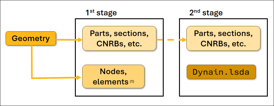
Because node and element definitions are specified in this file, you must modify the keyword file for the subsequent analysis to avoid double definitions. It is best practice to partition the geometry keyword file into two parts: one part with node and element definitions, and one part with the remaining keywords (parts, sections, constraints, sets, and more) as shown in the previous figure.
Note: Not all element types will be included in the dynain.lsda file.
Table 10.1: List of dynain.lsda entities
| Output to dynain.lsda | Not output to dynain.lsda |
|---|---|
*NODE, *ELEMENT_... | *ELEMENT_MASS |
*CONSTRAINED_ADAPTIVITY | *CONSTRAINED_{OPTION} |
*BOUNDARY_SPC(1) | *LOAD_... |
*INITIAL_STRESS_... | *MAT_... |
*INITIAL_FOAM_REF... | *DEFINE_... |
| Contact state | *CONTACT_ |
*PART, *SECTION | |
*SET_... |
Note:
(1) SPC constraints output limits flexibility. To prevent this, use the *INTERFACE_SPRINGBACK_EXCLUDE keyword. |
The keyword file format may vary. A keyword (pseudo-code) example for a first analysis follows:
*KEYWORD
*INCLUDE
geo001_parts_sections.key
*INCLUDE
geo001_node_elements.key
*INCLUDE
control_cards...
*CONTROL_TERMINATION
                Define end time of the simulation
*CONTACT_AUTOMATIC_SINGLE_SURFACE_MORTAR_ID
101Global contact
...
*LOAD_...
                Define nodal loads etc.
*BOUNDARY_...
                Data line to prescribe boundary conditions
*INTERFACE_SPRINGBACK_LSDYNA
                Parameters for requesting a dynain.lsda - file
*TITLE
                Simulation title
*END
The following is a keyword example for subsequent analyses:
*KEYWORD
*INCLUDE
geo001_parts_sections.key
*INCLUDE
dynain.lsda
*INCLUDE
control_cards...
*CONTROL_TERMINATION
Define end time of the simulation
*CONTACT_AUTOMATIC_SINGLE_SURFACE_MORTAR_ID
101Global contact
...
*LOAD_...
Define nodal loads etc.
*BOUNDARY_...
Data line to prescribe boundary conditions.
*INTERFACE_SPRINGBACK_LSDYNA
Parameters for requesting a dynain.lsda file
*TITLE
Simulation title
*END
The dynain.lsda file is recognized automatically by version 4.8 of LS-PrePost. After obtaining this file, you have the option to open and visually inspecting the subsequent analyses.
The IDs of contacts in the subsequent analysis must match the first analysis for the contact state to intiate properly.
A template for requesting a binary dynain file follows:
*SET_PART_LIST_GENERATE_TITLE
All parts for dynain.lsda
338
1 99999999
*INTERFACE_SPRINGBACK_LSDYNA
$#    psid     nshv    ftype       _     ftensr     nthhsv   rflag   intstrn
       338      999        3       0          0          0       1         0
$#    optc     sldo     ncyc  fsplit     ndflag      cflag   hflag
OPTCARD           0        0       0          1          1       1
*INTERFACE_SPRINGBACK_EXCLUDE
$#                                                                   kwdname
BOUNDARY_SPC_NODE
The part set ID does not always indicate all the model parts, and the parts included in the ID is affected by the nature of the subsequent analyses.
The last exclude option supresses the printing of boundary conditions to the
dynain.lsda file. By supressing that, it gives the option to
keep the same boundary conditions or redefine it for the following analysis. In each
analysis, the simulation time starts from T = 0 and ends at T =
endtime of *CONTROL_TERMINATION as defined in each
keyword file.
In most analyses, the dynain file is output at the end of the termination time. R12.0.0 and more recent versions of LS-DYNA allow you to create the dynain file using sense switches. In the folder where the simulation is running, create a file called d3kil (if it does not already exist) and enter one of the following switches:
SWBLS-DYNA writes a dynain file and continues to run.
SWCLS-DYNA writes a dynain file and restart files. The application continues to run.
SWDLS-DYNA writes a dynain file and restart files, but then terminates.
The resulting dynain file is based on the *INTERFACE_SPRINGBACK_LSDYNA keyword specifications.
For more information on sense switches, see the Getting Started section of Keyword Manual Vol. I.
Note: Nodal velocities and accelerations are not stored in dynain.lsda. This makes it less useful for transient dynamic analyses that are carried out via the multistage approach described in Combining dynain.lsda and *CASE for Multistage Analyses.
You can combine dynain.lsda restart options with the built-in case driver to automate the analysis of loading sequences. This allows you to run a sequence of load cases automatically. The application propagates state information between each analysis. You must include the *CASE_ keywords in the keyword file, and add case to the
execution line of the application when submitting the main job. See Appendix X of Keyword User's Manual Vol. I and [34] for details.
The following keywords sets up a basic sequence of analyses, starting with bolt pretensioning then X- and Y-loadings.
*KEYWORD
*CASE_BEGIN_1
*INCLUDE
    run_pretens.key
*CASE_END_1
*CASE_BEGIN_2
*INCLUDE
    case1.dynain.lsda
*INCLUDE
    run_xload.key
*CASE_END_2
*CASE_BEGIN_3
*INCLUDE
    case2.dynain.lsda
*INCLUDE
    run_yload.key
*CASE_END_3
*END
The *CASE_ keywords seperates the output files of each analysis
(d3plot, d3hsp,
binout, and so forth), and names them with the case ID as
the prefix like in the example files case1.d3hsp and
case2.d3plot.
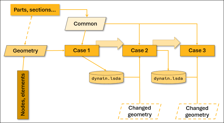
Keywords other than *CASE_BEGIN_N and *CASE_END_Nare common to all cases. This gives you the option to place the main model definition (such as control cards, boundaries, and contacts) in the common block, and limits each *CASE_ content block to the load-case specific keywords. The following
flowchart outlines the options for analyzing a sequence of load cases using dynain.lsda and LS-DYNA's *CASE functionality.
Note: The *CASE_ keywords must appear in the main keyword file (submitted to LS-DYNA as i=main_keyword.k). The *CASE_ keywords can't appear in the include files (referenced by the main keyword file using *INCLUDE).
The following figure shows an L-shaped bracket assembly that is subjected initially to bolt pretensioning, followed by loadings in the X and Y directions.
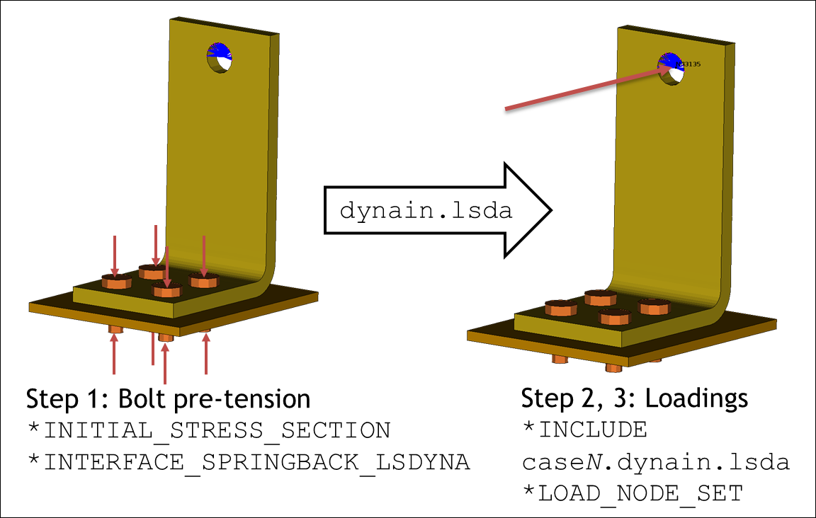
In this example, the main run file is L_bracket_dynain.key, and the analysis of these load stages is set up as a sequence of three cases as described in Table 10.2: CASE analysis of L-bracket assembly. This anlysis information is propogated between each analyses using the dynain.lsda binary format files.
Table 10.2: CASE analysis of L-bracket assembly
| Case # | Load description | Simulation time |
|---|---|---|
| 1 | Bolt pretensioning | 0 🡪 1 |
| 2 | X loading … | 0 🡪 1 |
| and unloading | 1 🡪 2 | |
| 3 | Y loading … | 0 🡪 1 |
| and unloading | 1 🡪 2 |
The application also sets up an all-in-one analysis for reference, and the main run file is L_bracket_allin1.key. The loadings in this analysis vary with simulation time according to Table 10.3: All-in-one analysis for L-bracket assembly.
Table 10.3: All-in-one analysis for L-bracket assembly
| Load description | Simulation time |
|---|---|
| Bolt pretensioning | 0 🡪 1 |
| X loading … | 1 🡪 2 |
| and unloading | 2 🡪 3 |
| Y loading … | 3 🡪 4 |
| and unloading | 4 🡪 5 |
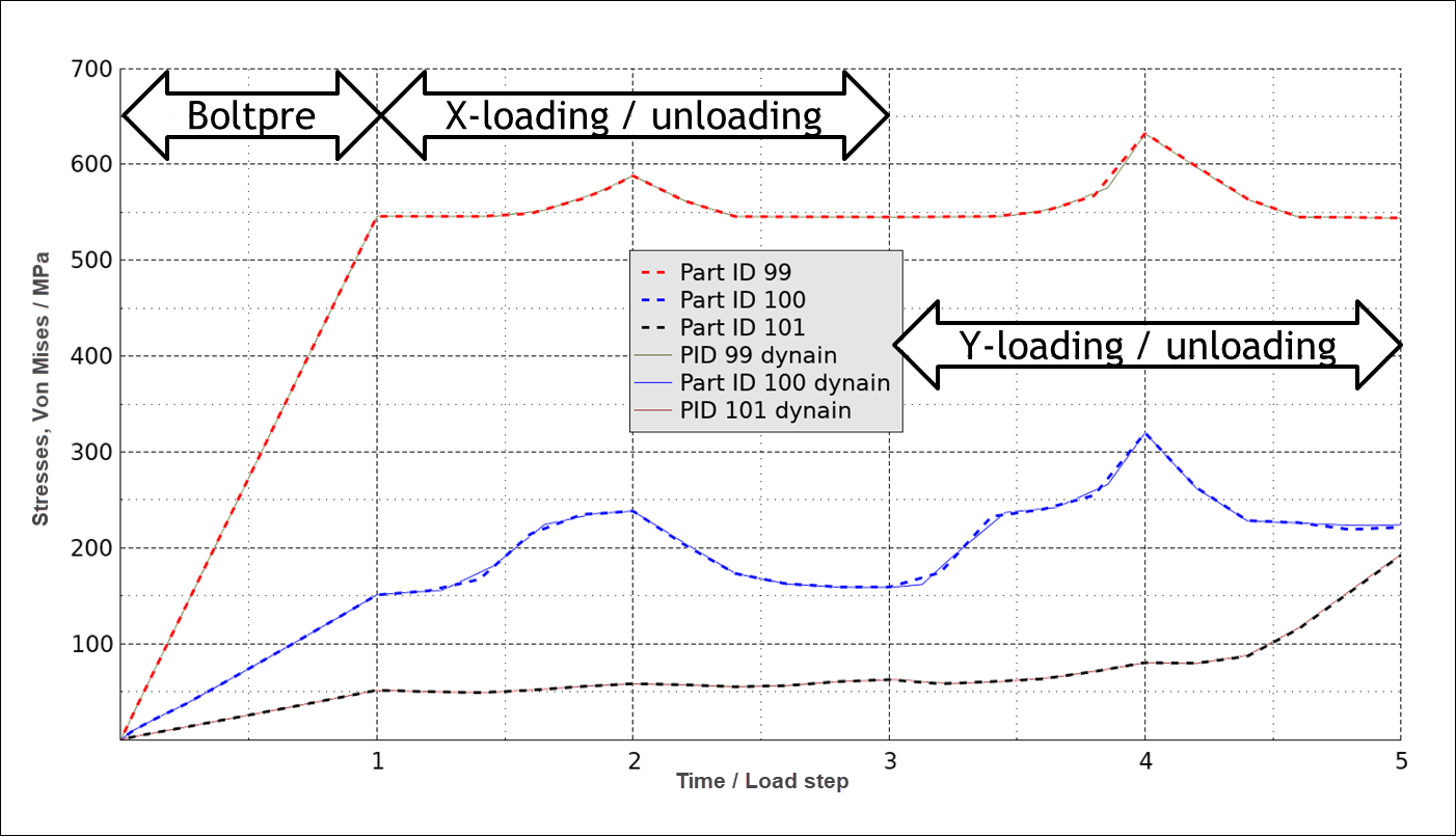
The following figure compares the history of each part's peak effective stress for
the two analysis approaches (all-in-one analysis and multistage analysis). The
all-in-one analysis is shown in dashed lines. The multistage analysis uses
dynain.lsda and *CASE, and is shown in solid
lines. The results from the multistage approach are time-shifted to match the
all-in-one analysis. The general agreement is very good, indicating how well the
dynain.lsda file carries the state information over between
analyses.
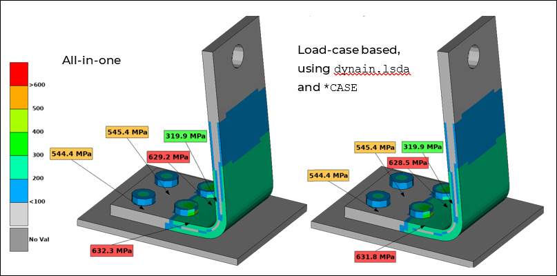
The next figure compares fringe plots of the effective stress at the peak Y-loading between the two analysis approaches. In the figure, the all-in-one analysis is on the left, and the load-case analysis is on the right. There are only very small differences (0.1 %) between the two.