For many dynamic analysis types (such as noise, vibration and harshness (NVH) and earthquake analyses), it is convenient to study the response of a structure in the frequency domain instead of the time domain. Several frequency domain analysis types are available in LS-DYNA:
calculation of frequency response functions
steady state dynamics
response spectrum analysis
random vibration analysis
FEM and BEM acoustics
Prior to version R11, these analyses were performed using a modal basis, which implies that an eigenfrequency analysis is required. See Eigenfrequency Analysis.
If stresses are of interest in a frequency domain analyses (for example, for random
vibration fatigue or steady state dynamics analyses), they must already have been
calculated during the eigenfrequency analysis. This can be achieved by setting the
parameter MSTRES = 1 on card 2 of the
*CONTROL_IMPLICIT_EIGENVALUE keyword. The eigenfrequency analysis can
be a part of the frequency domain analysis, or performed in a separate, preceding
analysis. The d3eigv files must be in double precision format. From
R11 of SMP, a direct solution for steady state dynamics is available by the keyword(s)
*FREQUENCY_DOMAIN_SSD_DIRECT and
*FREQUENCY_DOMAIN_SSD_DIRECT_FREQUENCY_DEPENDENT.
Note that the frequency domain analyses are linear, which means that the same restrictions as mentioned in Linear Static Analysis apply (see Sliding Contacts in Eigenvalue Analyses and Linear Implicit Analyses). The appropriate control card file is control_cards_linear.key.
An overview of the frequency domain analysis capabilities is presented in [8] and [43]. A thorough description is given in [9]. For more examples of NVH analyses in LS-DYNA, seehttps://lsdyna.ansys.com/knowledge-base/nvh-fatigue/.
Related keywords begin with *FREQUENCY_DOMAIN (see Keyword Manual Vol. I) and involve almost
the complete problem definition on several cards (including loadings and damping
definitions). Output for the different frequency domain analysis types can be requested
by using the keywords
*DATABASE_FREQUENCY_BINARY_OPTION, and from R10
also the keyword
*DATABASE_FREQUENCY_ASCII_OPTION.
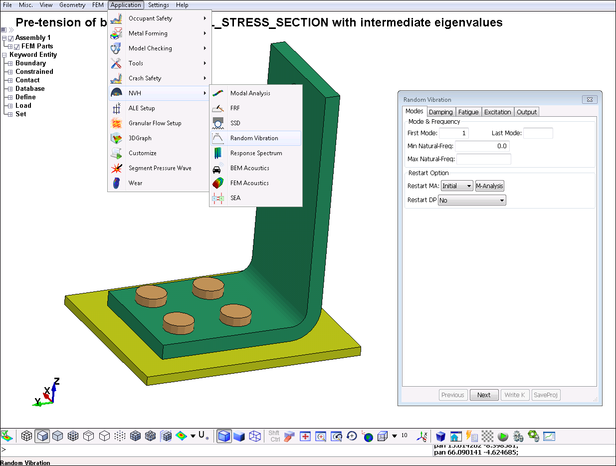
LS-PrePost version 4.3 and later includes a wizard for setting up different types of frequency domain analyses. It is accessed from the top menu bar, > , as shown in the following figure. LS-PrePost also has dedicated functionality (the NVH Fringe component) for convenient post-processing of frequency domain results.
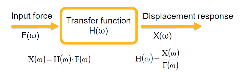
Frequency response functions (FRFs) of a dynamic system can be seen as the transfer functions between the excitation in one point and the response in another point, as shown in the following figure. (See [8].)
To calculate FRFs (such as dynamic stiffness or impedance), use the keyword
*FREQUENCY_DOMAIN_FRF. The excitation can be base velocity, base
acceleration, base displacement, nodal force, or pressure on a segment set. The
response can be velocity, acceleration, displacement, or nodal force. The output is
given in the ASCII files frf_amplitude and
frf_angle. To compute the real and imaginary parts
(frf_real and frf_imag), set the
parameter OUTPUT = 1.
A template for the frequency response function keyword follows:
*FREQUENCY_DOMAIN_FRF
Card 1: Define excitation and select modes
Card 2: Define damping
Card 3: Define the response
Card 4: Define output parameters
Steady state dynamics obtains the linearized steady state response of a structure
subjected to harmonic excitation, such as a fuel pump attached to a vibrating
engine. Use the keyword *FREQUENCY_DOMAIN_SSD to activate steady state
dynamics. If stresses are of interest, set the parameter MSTRES
= 1 on card 2 of the *CONTROL_IMPLICIT_EIGENVALUE keyword in the
preceding eigenfrequency analysis.
Steady State Dynamics Output
Output from a steady state dynamics analysis can be obtained as 3D binary plot
files d3ssd (containing displacements, stresses, and so forth,
similar to d3plot) and as ASCII history database files. The
output frequencies for the d3ssd databases are specified using
the *DATABASE_FREQUENCY_BINARY_D3SSD keyword. This keyword controls
which frequencies are analyzed in the SSD analysis. Linear, logarithmic or biased
spacing of output frequencies are possible.
Nodal and element history output are specified in the same way as for a
time-domain analysis: by using
*DATABASE_HISTORY_OPTION. The output files for
steady state dynamics are nodout_ssd and
elout_ssd. From R10, the keyword
*DATABASE_FREQUENCY_ASCII_OPTION can be used
to specify separate or additional output frequencies for these files.
Using the Large Mass Method for Enforced Motion
In LS-DYNA R9 and earlier, enforced nodal motion (acceleration, velocity,
displacement) is not explicitly implemented for steady state dynamics. If this type
of excitation is desired, the large mass method can be used. A very large mass
𝑚𝐿 (recommended is
106 times the total mass of the structure) is then
applied to the nodes where the enforced motion is applied, using the keyword
*ELEMENT_MASS_{OPTION}. The desired motion is
achieved by application of a corresponding force p as follows:
For nodal acceleration ü, 𝑝 = 𝑚𝐿ü
For nodal velocity 𝑢̇, 𝑝 = 𝑖𝜔𝑚𝐿𝑢̇
For nodal displacement 𝑢, 𝑝 = −𝜔2𝑚𝐿𝑢
Note that no other boundary conditions (*BOUNDARY_SPC or
*BOUNDARY_PRESCRIBED_MOTION) in the direction of the desired motion
can be applied to the nodes where an enforced motion is to be applied by use of the
large mass method. The corresponding rigid body modes must be included in the
consecutive frequency domain analyses in order to obtain the desired result. The
application of the large masses may alter the eigenfrequencies or mode order, which
means that care shall be taken when selecting the eigenmodes.
From LS-DYNA R10, the large mass method has been semi-automated. The large mass
per node is specified via the keyword *CONTROL_FREQUENCY_DOMAIN.
LS-DYNA will convert the prescribed velocity, acceleration, or displacement
(VAD = 5 - 7) to the appropriate nodal force. You must
still add the actual mass elements
(*ELEMENT_MASS_{OPTION}). The excitation input
type codes have been changed from R9 to R10 as shown in the following table.
Table 4.1: Excitation Input Type Codes
| VAD | LS-DYNA R9 | LS-DYNA R10 and later |
|---|---|---|
| 0 | Nodal force | |
| 1 | Pressure | |
| 2 | Base acceleration | Base velocity |
| 3 | Enforced velocity(1) | Base acceleration |
| 4 | Enforced acceleration(1) | Base displacement |
| 5 | Enforced displacement(1) | Enforced velocity(2) |
| 6 | N/A | Enforced acceleration(2) |
| 7 | N/A | Enforced displacement(2) |
Notes:
| (1) Not explicitly implemented. |
| (2) Semi-automatic implementation by the large-mass method. |
Steady State Dynamics Template
A template for a steady state dynamics analysis follows:
*FREQUENCY_DOMAIN_SSD
Card 1: Select modes to be used in the analysis
Card 2: Define damping
Card 3: Define output for subsequent acoustic analysis
Card 4: Define the excitations (repeat if multiple excitations are
                    present)
*DATABASE_FREQUENCY_BINARY_D3SSD
Define frequency range, spacing etc. for output
*ELEMENT_MASS_{OPTION}
Define masses for enforced motion by the large mass
                method
For each excitation, two load curves are used (LC1 and LC2 of Card 4) for defining amplitude and phase (or real and imaginary component) as a function of frequency are required. These load curves must have the same number of abscissa values.
From R9.0.1[6], the _FATIGUE option for steady state dynamics analyses also computes the fatigue damage due to the dynamic load case(s). The load duration for each frequency must be specified as a load using the parameter LCFTG (position 1 of Card 8) from R12. For versions prior to R12,
use LC3 on position 7 of Card 4. The fatigue properties (S-N-curves) for each material, respectively, must be specified using the keyword *MAT_ADD_FATIGUE.
Stresses are required for the fatigue analysis. This means that you must set the
parameter MSTRES = 1 on card 2 of the
*CONTROL_IMPLICIT_EIGENVALUE keyword in the preceding
eigenfrequency analysis.
*DATABASE_FREQUENCY_BINARY_D3FTG must be specified in order to get 3D
binary plot files for visualization of fatigue analysis results.
Consider switching to Lobatto quadrature for shell elements when performing fatigue analyses, see Shell Elements. This provides integration points exactly on the inner/outer surface.
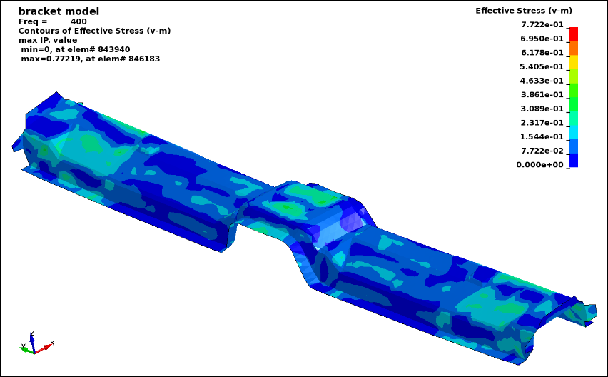
Steady State Dynamics Example: Fatigue in a Bracket
A basic example of a steady state dynamics analysis of a bracket, including fatigue evaluation, is available in the example file ssd_fatigue001.key. The figure below shows the effective stress (von Mises) response at 400 Hz.
From R11.1 of LS-DYNA, a direct solution option is available for steady state
dynamics, activated by the keyword *FREQUENCY_DOMAIN_SSD_DIRECT (or
*FREQUENCY_DOMAIN_SSD_DIRECT_FREQUENCY_DEPENDENT for cases with
frequency dependent material properties). Using a direct solution approach may be
advantageous if only a few excitation frequencies of a large model are to be
analyzed, since in such a case the eigenvalue analysis may be quite time-consuming.
To get output of stresses, set the variable ISTRESS = 1 on Card 3 of the *FREQUENCY_DOMAIN_SSD_DIRECT keyword. The direct solution option is only available in SMP (up to and including R15.0.0). See [31] for further details.
Random vibration is non-deterministic motion, such as a vehicle riding on a rough
road. Structures subjected to random vibrations are usually studied using
statistical or probabilistic approaches. The power spectral density (PSD) is
commonly used to specify a random vibration process [8]. In LS-DYNA, a stationary random process, meaning that the
statistics describing the process does not change over time, is assumed. The keyword
*FREQUENCY_DOMAIN_RANDOM_VIBRATION activates the random vibration
analysis, and by adding the option _FATIGUE also the fatigue damage of
a component subjected to the random process can be evaluated. Many different fatigue
evaluation methods are implemented in LS-DYNA, including:
Dirlik's method based on the 4 moments of PSD
Wirschinig's method
The narrow band method
Steinberg's three-band technique, considering the number of stress cycles at the levels 1σ, 2σ, and 3σ levels
Dirlik's method is considered to be the most useful for general purpose applications [8].
Fatigue Analysis
Stresses are required for the fatigue analysis. You must set the parameter
MSTRES = 1 on card 2 of the
*CONTROL_IMPLICIT_EIGENVALUE keyword in the preceding
eigenfrequency analysis.
You must request the binary database d3rms using the
*DATABASE_FREQUENCY_BINARY_D3RMS keyword. You must use the
*DATABASE_FREQUENCY_BINARY_D3FTG keyword to get 3D binary plot
files for visualization of fatigue analysis results.
Consider switching to Lobatto quadrature for shell elements when performing fatigue analyses (see Discrete Elements, Springs, and Dashpots) to get integration points exactly on the inner/outer surface and activate output of individual shell in-plane integration points (see Solid Elements).
Random Vibration Analysis
For a random vibration analysis, the PSD of displacements, velocities, accelerations and stresses are output in the 3D binary database d3psd. In addition, the root mean square results for the same quantities are output in the 3D binary database d3rms. Nodal and element PSD results are available in the binout results elout_psd and nodout_psd. Fatigue results are output as stress components in the 3D binary database as shown in Table 4.2: Fatigue Analysis Results. LS-PrePost will present the correct result labels when a d3ftg file is opened.
The irregularity factor is a real number from 0 to 1, where a sine wave has an irregularity factor of 1 and white noise has an irregularity factor of 0. The lower this value, the closer the process is to the broad band case. The higher the value, the closer the process is to the narrow band case.
Table 4.2: Fatigue Analysis Results
| Result / component | Fatigue analysis results | Comment |
|---|---|---|
| σXX | Cumulative damage ratio | |
| σYY | Expected fatigue life | |
| σZZ | Zero-crossing frequency | |
| σXY | Peak-crossing frequency | |
| σYZ | Irregularity factor | |
| σXZ | Expected fatigue life | From R12 |
| εp(1) | Counted cycles | From R12 |
Note:
| (1) Accumulated effective plastic strain. |
Random Vibration and Fatigue Analysis Template
A template for a random vibration fatigue analysis follows:
*FREQUENCY_DOMAIN_RANDOM_VIBRATION_FATIGUE
Card 1: Select modes
Card 2: Define damping. Note: This is mandatory. Some damping must be specified.
Card 3: Define loading type and the number of PSD loadings and fatigue
                    data (SN-curves) definitions
Card 4: Define exposure time and type of S-N curves
Card 5: Define the excitation PSDs (repeat if multiple excitations are
                    present)
Card 6: Define the fatigue data for each PID
*DATABASE_FREQUENCY_BINARY_D3PSD
Define frequency range, spacing etc. for output
*DATABASE_FREQUENCY_BINARY_D3RMS
1,
*DATABASE_FREQUENCY_BINARY_D3FTG
1,
Important: Be aware of the following when using this template:
The excitation PSDs must be defined for positive frequencies only. Specifying zero or negative frequencies in the load curve definitions leads to errors.
You must include some kind of damping. Card 2 cannot be left blank or assigned values of zero.
From R9.0.1, the fatigue properties (S-N-curves) for each material, respectively, may instead be specified using the keyword *MAT_ADD_FATIGUE if the variable NFTG on card 5 is set to -999.
In random vibration analysis, special care must be taken when computing the RMS of the von Mises effective stress, it cannot be obtained directly from the RMS of the stress components. In LS-DYNA, the method described in [12] is implemented. The von Mises stress is stored in d3psd and d3rms instead of plastic strain. LS-PrePost (version 4.3 and later) displays this value instead of computing it from stress components[7].
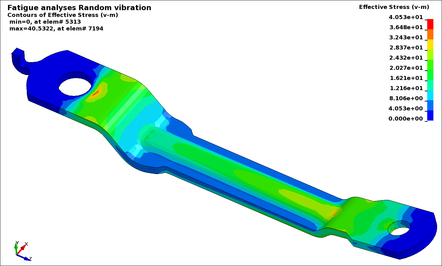
Random Vibration and Fatigue Analysis Example: Link Arm
A basic example of random vibration analysis of a link arm, including fatigue evaluation, is available in keyword file set_4.key. The following figure shows a plot of the RMS effective stress.