


(Part A) Learn how to set up and process a simulation using Coarse Grain Modeling (CGM) and import an *.f2r file into Rocky for 1-Way Fluent coupling.
(Part B) Learn how to identify when particle flow reaches a steady state, compare the mass flow between outputs, and build Custom Properties to estimate the work of shear forces.
The main purpose of this tutorial is to learn how to use Coarse-Graining to increase the particle size while maintaining the system behavior, but using a reduced number of (larger) particles.
We will also learn how to export Ansys Fluent results as an .f2r file (optional) and further couple this already-processed CFD simulation with our DEM simulation setup in Rocky.
The scenario considered is a pneumatic transport of micrometer-sized particles within a mixing tee.
You will learn how to:
(Optional) Export Fluent CFD results as an .f2r file
Import an .f2r file into Rocky
Use Coarse-Graining to scale-up the particle size (and reduce the processing time)
Collect Intensities data via Boundary Collisions Statistics
And you will use these programs and features:
(Optional) Ansys Fluent:
Export Solution to Rocky
Rocky:
Coarse-Graining
Fluent 1-Way Steady State coupling
Boundary Collision Statistics
This ADVANCED tutorial assumes that you are already with the Rocky user interface (UI) and Rocky project workflow.
If this is not the case, it is recommended that you complete at least Tutorials 01- 05 before beginning this tutorial.
Important: Even though this tutorial makes use of CFD results from Ansys Fluent, you are not required to have a Fluent license. Specifically:
If you do not have Ansys Fluent, you can skip the CFD setup steps and just use the provided results when you are ready to import them into Rocky.
(Optional) If you do have Ansys Fluent and want to process the CFD results yourself, ensure that you have a valid license for Ansys 2025 R2.
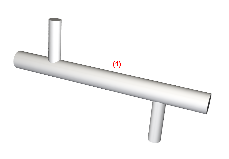
The geometry in this tutorial is composed of:
(1) Mixing Tee
In the tutorial directory, a .cas file containing this geometry can be found.
Note: If you are completing this tutorial without Ansys Fluent, please skip ahead to the Rocky setup steps, which begin on ROCKY PROJECT SETUP.
To set up the Fluent Case, do the following:
Download the
dem_tut17_files.zipfile here .Unzip
dem_tut17_files.zipto your working directory.Open Ansys Fluent.
From the Fluent Launcher, under Dimension, ensure that 3D is selected; also, under Solver Options, ensure that Double Precision is selected.
Important: Double Precision and 3D are required for coupling with Rocky.
From the Solution workspace, below Capability Level, select Case from the dropdown list.
From the Browsing Case File dialog, navigate to the geometry folder that you previously downloaded, select the mixing_tee_fluent.cas file, and then click Open.
Under Parallel, set the number of Solver Processes.
Click Start.
In this tutorial, we will export an .f2r (Fluent to Rocky) file, which requires prior installation of a special Fluent/Rocky export component.
Ensure that you have this component by doing the following:
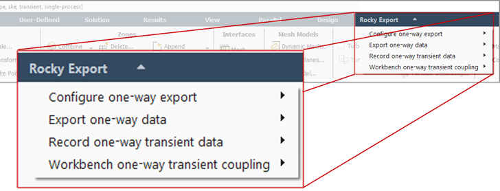
At the top of the Fluent program window, see if you have listed the Rocky Export menu (as shown).
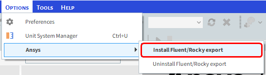
If you do not see this menu in Fluent, then do the following: From the Rocky program's Options menu, point to Ansys and then click Install Fluent/Rocky export (as shown).
Tip: It is also possible to couple Fluent and Rocky through the Ansys Workbench program. (See also Tutorial - Windshifter).
From the Fluent Outline View tree panel, under Solution, double-click Run Calculation.
From the Run Calculation Task Page, click Calculate. If you are asked to initialize the case, click Yes.
After the calculation completes, from the Rocky Export menu, point to Export one-way data, and then click Export current data to Rocky (as shown).
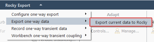
The .f2r file will be automatically saved in the same location as the .cas file.
Close Fluent. (It is not necessary to save the case for this tutorial.)
Note: If you are completing this tutorial without Ansys Fluent, you can begin the tutorial from this step.
Download the
dem_tut17_files.zipfile here .Unzip
dem_tut17_files.zipto your working directory.Open Rocky 2025 R2
Create a new project.
Save the empty project to a location of your choosing.
For this tutorial, we want to do all of the following:
Enable Coarse-Graining to help with simulating micron-sized particles.
Use the Boundary Collision Statistics module to collect Intensities. This data can be useful for analyzing impact wear and power draw.
Import geometries via the same Fluent .cas file we used earlier (in the optional steps).
Let's start by learning about Coarse-Graining.
Coarse-Graining enables you to increase the original particle size to study the system behavior using a feasible number of (larger) particles.
This physics accomplishes this by doing the following:
Scales-up the particle size, which reduces the number of particles that need to be processed, thereby lowering the computational load.
Adjusts the particle interactions of the newly scaled-up particles so that the larger particles behave more like the smaller particles they represent.
Rather than creating an impractical case involving, perhaps, hundreds of millions of tiny particles, Coarse-Graining makes it possible to analyze an approximated case with a more manageable particle count all without sacrificing accuracy.
Note: The Coarse-Graining model used in Rocky is based on the work of Bierwisch et al. (2009). Refer to the Rocky DEM Technical Manual for further details.
To apply Coarse-Graining in Rocky, you specify a unique CGM Scale Factor for each Particle set.
This factor is multiplied by the original particle size to obtain an easier-to-process scaled-up particle, called a parcel.
The job of a single, scaled-up parcel is to represent many original-sized particles while retaining the same interaction behaviors as the smaller particles it represents.
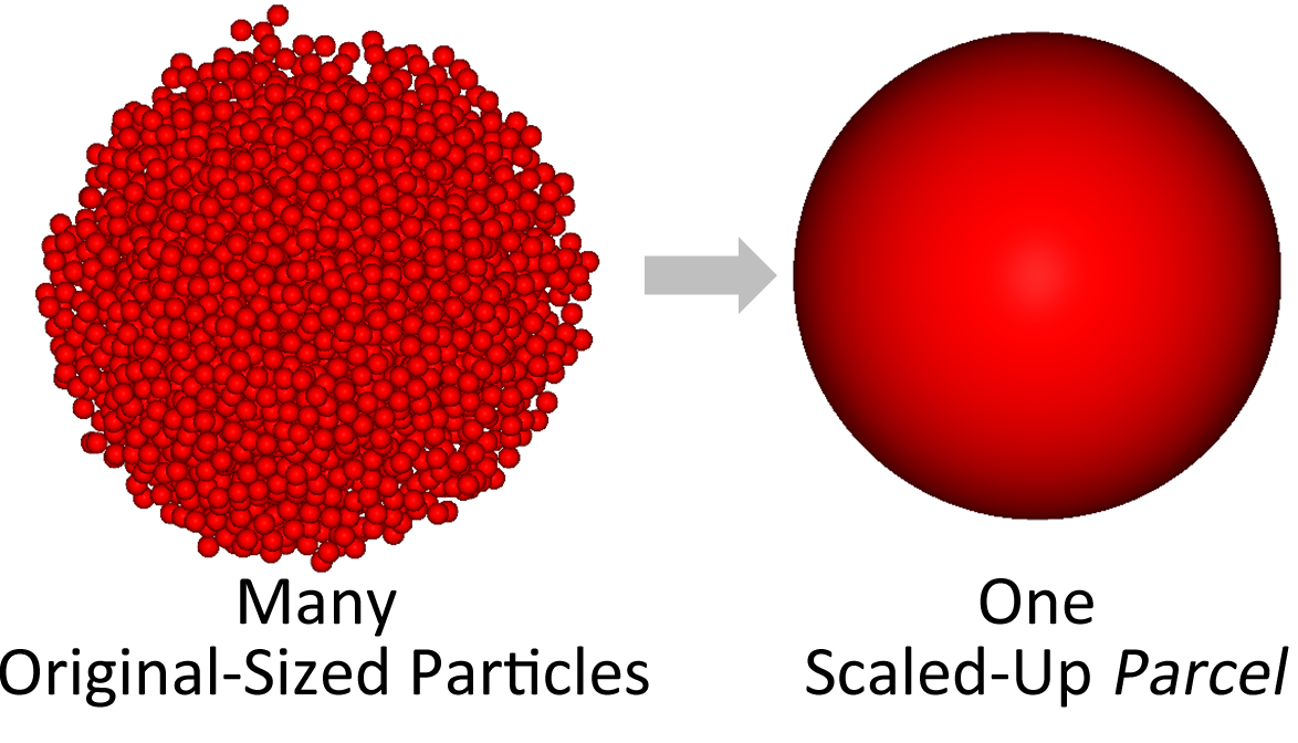
To achieve this latter goal, the CGM Scale Factor is also used to adjust the contact, adhesion, thermal, drag, and other interaction properties of the scaled-up parcel so that it behaves more like the original-sized particles.
Use the information in the table below to start setting up your Rocky project.
Tip: If you run into settings or procedures in these tables that you are not yet familiar with, please refer to the Rocky User Manual and/or other Tutorials (via the Introductory Tutorials and Advanced Tutorials) to find the detailed instructions you need.
Step Data Entity Editors Location Parameter or Action Settings A Study Study Study Name CGM Study B Physics Physics | Gravity Y-direction 0 [m/s2] Z-direction -9.81 [m/s2] Physics | Momentum Numerical Softening Factor 0.1 [ - ] Physics | Coarse-Graining Enable Coarse-Graining (Enabled) C Modules Modules Boundary Collision Statistics (Enabled) D Modules ﹂Boundary Collision Statistics
Boundary Collision Statistics Intensities (Enabled) E Geometries Import Wall mixing_tee_fluent.cas with "m" for Import Unit Note: "CGM" refers to Coarse Grain Modeling.
Five separate geometry components are imported.
For this tutorial, we need only the wall geometry.
From the Data panel, multi-select the two inlet and two outlet geometry components.
Right-click the selection of four items, and then click Remove Geometries.
Important: Only the wall geometry component should remain at this point.
Next, we will define a surface that will be used as an inlet to release the particles into the domain.
We will also be creating a spherical-shaped particle group with a range of three different sizes.
Note that we will be using default values for both the Materials and Materials Interactions settings.
Use the information in the table below to continue setting up your Rocky project.
Step Data Entity Editors Location Parameter or Action Settings A Geometries Create Circular Surface B Geometries ﹂Circular Surface <01>
Circular Surface Center Coordinates 0, 0, 0.36 [m] Max Radius 0.048 [m] Angle 90 [dega] C Particles Create Particle
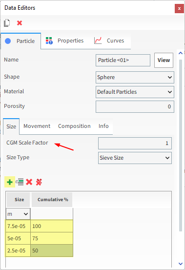
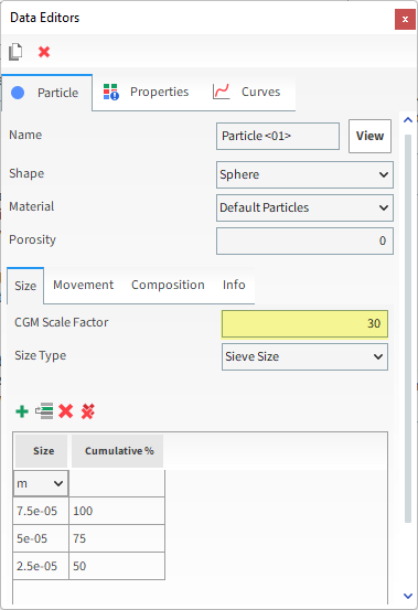
From the Data Editors panel, on the main Particle tab, select the Size sub-tab, and then check the CGM Scale Factor:
For now, we will leave the CGM Scale Factor as 1 (particles equal to the original size).
Later in this tutorial, we will compare the particles count for CGM Scale Factors of 1 and 30.
Click the Add button (green plus) twice to add two more particle size rows.
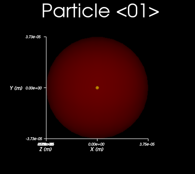
For each row, define the Size (and Units) and Cumulative % values (as shown). Click View.
Reminder: The Particles Details window always reflects the size of the largest particle in the set. (In this case 7.5e-05 m.)
For the Inlets and Outlets step, we will create a Particle Inlet.
Use the information in the table below to continue setting up your Rocky project.
Step Data Entity Editors Location Parameter or Action Settings A Inlets and Outlets Create Particle Inlet B Inputs ﹂Particle Inlet <01>
Particle Inlet Entry Point Circular Surface <01> ⯆ Particle Inlet | Particles Add row (x1) (1) Particle | Mass Flow Rate Particle <01> ⯆ @ 0.1 [t/h] … | Time Stop 1 [s] … | Entry Target Normal Velocity (Enabled) 4 [m/s]
Now, let's see how many particles are estimated if we simulate at this (original) particle size.
From the Data panel, click Inlets and Outlets.
From the Data Editors panel, on the Info tab, view the estimated number of particles.
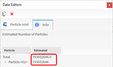
Note: This estimate is made using the Inlet parameters (e.g. Start and Stop Times, Target Velocity and Surface Dimensions) and the Particles parameters (e.g. Size and Material).
For this tutorial, we will assume that we do not have the computational resources to process the hundreds of millions of estimated particles.
To make this simulation more reasonable to process, we will now set a higher CGM Scale Factor to reduce the particle count.
From the Data panel, under Particles, click Particle <01>.
From the Data Editors panel, on the Size sub-tab, increase the CGM Scale Factor.
By viewing again the particle estimates in Inlets and Outlets, a significant reduction of particles can be seen.
From the Data panel, click Inlets and Outlets.
From the Data Editors panel, on the Info tab, view the updated particle estimate.
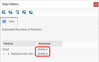
Now ranging in only the tens of thousands of particles, this case should be much easier to process. In addition, the corrections made by the Coarse-Graining will ensure that the interactions closely approximate those of the original case.
Important: As a reminder, the CGM factor f is multiplied by the particle diameter, which means that the parcel's volume and mass are f3 times bigger when compared with those from the original particle. The outcome is a reduction in the particle count by f3 times.
For this tutorial, an exaggerated CGM factor of 30 is used to speed up simulation time. However, note that an over-scaled CGM factor may cause unrealistic physical results and numerical instability (e.g. 2-Way Coupling cases).
For the CFD Coupling step, we will be importing some steady-state CFD results that were already processed in Fluent.
From the Study menu, enable the 1-Way Fluent CFD Coupling model.
From the Select Fluent 2 Rocky export file dialog, do one of the following:
If you completed the earlier steps in Ansys Fluent, navigate to the geometry folder, find the fluent_to_rocky.f2r file (which was generated by Ansys Fluent when you exported the results), and then click Open.
If you did not complete the earlier steps in Ansys Fluent, navigate to the geometry/cfd-one-way folder, select the mixing_tee_cfd.f2r file, and then click Open.
From the Data Editors panel, on the 1-Way Fluent | Interactions tab, enable the Turbulent Dispersion checkbox.
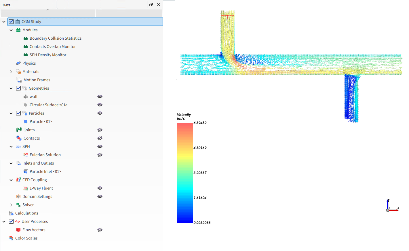
Now that the CFD results are within Rocky, you can visualize the nodes of the cell centroids making up the Fluent mesh.
Important: Given the amount of elements, showing all vectors for your CFD meshes is not considered good practice as it can freeze the Rocky interface.
A better practice is to create a thin slice of your mesh and show only the vectors within that slice.
Use the information in the table that follows to set up and visualize this slice.
Step Data Entity Editors Location Parameter or Action Settings A CFD Coupling ﹂1-Way Fluent
Create a Cube User Process B User Processes ﹂Cube <01>
Cube Name Flow Vectors Center 0.45, 0, 0 [m] Magnitude 1.7, 0.02, 0.9 [m] C User Processes ﹂Flow Vectors
Show in new 3D View D User Processes ﹂Flow Vectors
Coloring Vectors (Enabled) Vectors | Property Velocity ⯆ Vectors | Vector scale 0.025 [ - ] Vectors | Normalized vectors (Enabled)
The colored vectors show that the fluid enters the domain through two inlets, (left portion of the figure) and flow through two outlets (right portion of the figure).
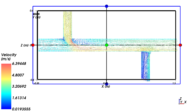
Tip: To see the vectors, you might need to make the wall geometry transparent or hidden.
Lastly, we need to define the Solver setup.
Use the information in the table that follows to finish your Rocky setup.
Step Data Entity Editors Location Parameter or Action Settings A Solver Solver | Time Simulation Duration 1 [s] Output Settings | Time Interval 0.01 [s] Solver | General Simulation Target CPU ⯆
With a 3D View window opened, your Data panel and Workspace should look similar to the below image.
From the Solver entity, click Start.
The Simulation Summary screen appears, then processing begins.
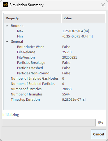
Tip: You can use the Auto Refresh checkbox to view in a 3D View window the results during processing.
This completes Part A of this tutorial.
Rocky was used to set up and process a Mixing Tee simulation.
During this tutorial, it was possible to:
(Optional) Export CFD results out of Ansys Fluent as an .f2r file.
In Rocky, set Boundary Collision Statistics in order to collect Intensities data.
Use Coarse-Graining to scale-up micro-sized particles for easier processing.
Import CFD results into Rocky by enabling 1-Way Fluent CFD Coupling.
What's Next? If you completed this tutorial successfully, then you are ready to move on to Part B and post-process this project.
The purpose of this tutorial is to use the results from the Mixing Tee simulation we set up and processed in Part A to analyze which wall regions are most susceptible to wear and discover how the particles are distributed between the outlets.
You will learn how to:
Identify when particle flow reaches a steady state
Compare the mass flow between the geometry outlets
Build Custom Properties to estimate the work of shear forces
And you will use these features:
Time Plots
Histograms
User Processes, including:
Cubes
Particles Time Selections
Filter
Particles Trajectory
Custom Properties
This ADVANCED tutorial assumes that you are already with the Rocky user interface (UI) and Rocky project workflow.
If this is not the case, it is recommended that you complete at least Tutorials 01- 05 before beginning this tutorial.
Important: Even though this tutorial makes use of CFD results from Ansys Fluent, you are not required to own a Fluent license in order to complete this tutorial.
If you completed Part A of this tutorial, ensure that Rocky project is open. (Part B will continue from where Part A left off.)
If you did not complete Part A, do all of the following:
Download the
dem_tut17_files.zipfile here .Unzip
dem_tut17_files.zipto your working directory.Open Rocky 2025 R2
Important: To make use of the Rocky project file provided, you must have Rocky 2025 R2 or later. If you have an earlier version of Rocky, please upgrade Rocky to the latest version, or complete Part A from scratch.
From the Rocky program, click the Open Project button, find the tutorial_17_A_pre-processing folder, open the tutorial_17_A_pre-processing.rocky file.
Process the simulation. (From the Data panel, select Solver and then from the Data Editors panel, click the Start button.)
With the processing complete, we can now analyze the results.
In order to perform statistical analysis, it is necessary to select a period of time in which the amount of particles inside the mixing tee remains stable.
We will do this by measuring the Particles Count curve over time.
Use the information in the table below to create this plot.
Step Item Location Parameter or Action Settings A Window (menu) Create a New Time Plot B Particles Curves | Particles Count Drag and drop onto open Time Plot <01> window
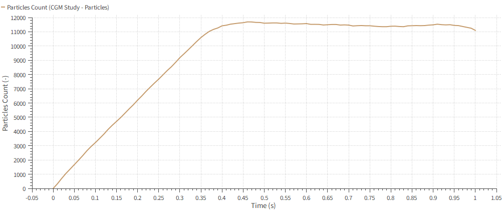
The resulting time plot shows that after approximately 0.5 seconds, the amount of particles inside the domain remains stable.
The range between 0.5 s and 1.0 s is a period of continuous operation of the equipment, and could be used for a statistical analysis.
We next want to compare the mass flow between the two outlets and understand how the particles separation occurs.
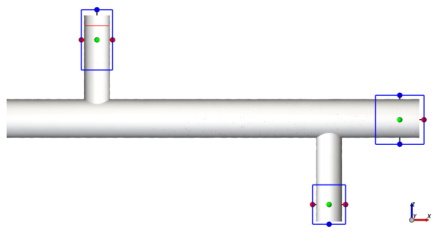
We will therefore define three Cube User Processes; one for the inlet and another two for the outlets.
Use the information in the tables that follow to define these Cubes.
Step Data Entity Editors Location Parameter or Action Settings A Particles Create a Cube User Process B User Processes ﹂Cube <01>
Cube Name Inlet Cube Center 0, 0, 0.305 [m] Magnitude 0.121, 0.157, 0.234 [m] C Particles Create a Cube User Process D User Processes ﹂Cube <01>
Cube Name Outlet Cube (Downwards) Center 0.9, 0, -0.334 [m] Magnitude 0.128, 0.157, 0.153 [m] E Particles Create a Cube User Process F User Processes ﹂Cube <01>
Cube Name Outlet Cube (Main) Center 1.174, 0, -0.005 [m] Magnitude 0.188, 0.157, 0.19 [m]
It is now possible to visualize the cubes in a 3D View.
In order to measure the total mass that passed through each cube once a steady state is reached (from 0.5 s on), we will create a Particles Time Selection process for each Cube.
Use the information in the tables that follow to define these processes.
Step Data Entity Editors Location Parameter or Action Settings A User Processes ﹂Inlet Cube
Create a Particles Time Selection User Process B User Processes ﹂Particles Time Selection <01>
Time Selection Name Inlet Measurement Domain Range Time Range ⯆ Initial 0.5 [s] Final 1 [s] C User Processes ﹂Outlet Cube (Downwards)
Create a Particles Time Selection User Process D User Processes ﹂Particles Time Selection <01>
Time Selection Name Outlet Measurements (Downwards) Domain Range Time Range ⯆ Initial 0.5 [s] Final 1 [s] E User Processes ﹂Outlet Cube (Main)
Create a Particles Time Selection User Process F User Processes ﹂Particles Time Selection <01>
Time Selection Name Outlet Measurement (Main) Domain Range Time Range⯆ Initial 0.5 [s] Final 1 [s]
Next, we will build a Histogram comparing the total mass and particle sizes between each Cube.
Use the information in the table below to create this plot.
Step Item Location Parameter or Action Settings A Window (menu) Create a New Histogram B User Processes ﹂Inlet Measurement
Properties | Particle Size Drag and drop onto open Histogram <01> window C User Processes ﹂Outlet Measurement (Downward)
D User Processes ﹂Outlet Measurement (Main)
E Histogram (window) Configure histogram (button) F Configure Histogram (dialog box) Weight Particle Mass ⯆ Number of Bins 3 Percent Values (Enabled)
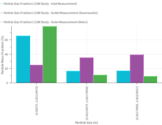
The Histogram shows the mass fraction of three ranges of particle sizes.
Note: Your histogram's bin colors might differ from the ones shown.
The dark red bins show that approximately 66% of the Inlet mass fraction is of small particles. The middle-sized and big particles have almost 17% of mass fraction each.
For the Main Outlet (orange bins), we have almost 80% of small particles mass fraction.
The blue bins (Downwards Outlet) show that the bigger the particle, the higher the mass fraction. In other words, bigger particles tend to flow downwards.
These results make sense as bigger particles (with greater mass) would require more energy to accelerate and escape the downwards outlet as the gravity force acts.
Note: Because we are using CGM, the particle sizes listed on the horizontal axis are 30 times bigger than the sizes we set in the Particles step.
In Rocky, you are able to visualize the effects of wear using the surface wear modification feature.
The wear law used in that feature takes into account the shear work on the geometry surface to predict how it will wear down over time.
Tip: For hands-on experience with surface wear modification, refer to Tutorial - SAG Mill and Tutorial - High Pressure Grinding Roll (HPGR).
However, for the case we are studying in this tutorial, the surface modification of the geometry would not be noticeable due to the short simulation time.
Instead, we can compute the total work done by the shear forces on each triangle surface and then verify which regions of the geometry have the highest shear work.
You might recall that in Part A, we enabled the collection of Intensities data for Boundary Collision Statistics. We can use that data to perform the shear work analysis.
A good approximation of it would be:
 | (17–1) |
Where:
 is a given time step.
  is the given boundary triangle.
  [J] is the Cumulative Shear Work from
0s to on the triangle.
[J] is the Cumulative Shear Work from
0s to on the triangle.  [W/m2] is the instantaneous Intensity : Shear on the triangle.
  [m2] is the Area :
Cell, which is the area of the triangle.
[m2] is the Area :
Cell, which is the area of the triangle.  is the time [s].
  [s] is the time between 2 outputs, which is dictated by the Output Frequency.
Let's now create a new custom Property that defines this.
First, we are going to calculate the Cumulative Intensity :
Shear, which is the  factor of the equation.
Use the information in the table below to create this custom property.
Step Item Location Parameter or Action Settings A Geometries ﹂wall
Properties Add new custom property (button) B Add new (dialog box) Name Cumulative Intensity: Shear Output unit W/m2 Inputs | Intensity: Shear (Enabled) C Custom Property (dialog box) Expression sum(A[:t+1])
The new Cumulative Intensity : Shear (Custom) property will appear on Properties tab under Transient.
Now, we are going to calculate the actual Cumulative Shear Work.
Use the information in the table below to create a second custom property.
Step Item Location Parameter or Action Settings A Geometries ﹂wall
Properties Add new custom property (button) B Add new (dialog box) Name Cumulative Shear Work Output unit J Inputs | Area: Cell (Enabled) Inputs | Cumulative Intensity: Shear (Custom) (Enabled) C Custom Property (dialog box) Expression A*B*OUTPUT_FREQUENCY
The new Cumulative Shear Work (Custom) property will appear on the Properties tab under Transient.
To visualize this new Cumulative Shear Work (Custom) property, drag-and-drop it onto a 3D View window.
To highlight the surface triangles that are most affected by wear, we will create a Filter User Process to filter them out.
Use the information in the table below to create a this Filter User Process.
Step Data Entity Editors Location Parameter or Action Settings A Geometries ﹂wall
Create a Filter User Process B User Processes ﹂Filter <01>
Property Property Cumulative Shear Work (Custom) ⯆ Mode Cut ⯆ Type Range ⯆ Minimum value 5e-06 [N.m] Maximum value 0.001 [N.m] Coloring Faces (Enabled) Faces | Property Cumulative Shear Work (Custom) ⯆ Faces | Show on Node? (Enabled) Edges (Cleared) From the Data panel, hide the two items under Geometries, every Cube and Particles Time Selection User Processes and show Particles by clicking their respective eye icons.
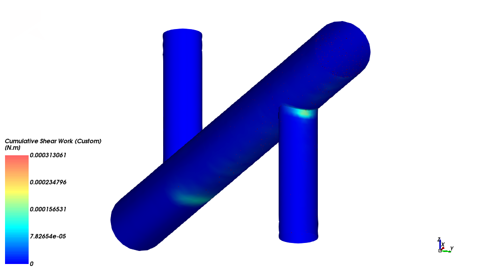
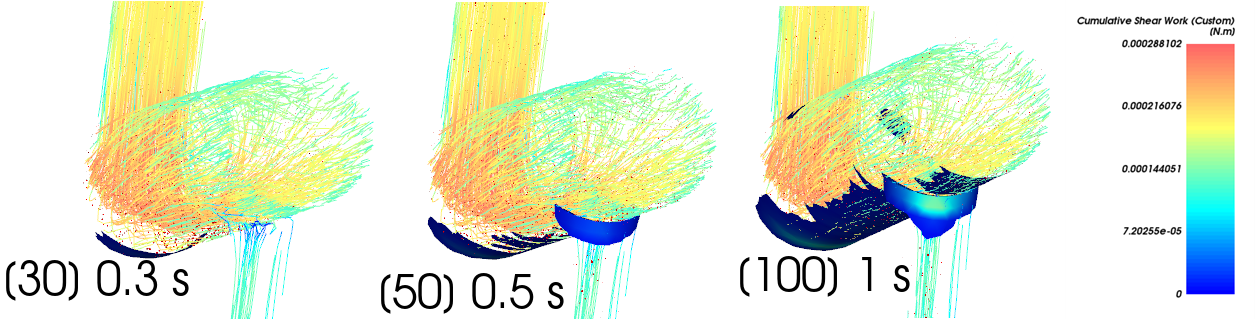
The results shown below are for the last output time: [100] 1 s
Now we will manually define the limits of the color scale and see how the surface wear changes over time.
From the Data panel, under Color Scales, select Cumulative Shear Work (Custom).
From the Data Editors panel, set the Limits options as User Defined, and then click the Compute limits in time range and set as "User defined" button.
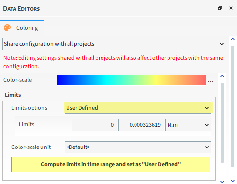
From the Calculate limits for the time range dialog, click OK.
Use the slider on the Time toolbar to see how the Cumulative Shear Work develops over time.
To get a better context of how the particles are interacting with the geometry, we can create a Particles Trajectory process:
From the Time toolbar, set the output time to [80] 0.8 s.
Use the information in the table below to create a this Particles Trajectory process.
Step Data Entity Editors Location Parameter or Action Settings A Particles Create a Particles Trajectory User Process B User Processes ﹂Particles Trajectory <01>
Particle Trajectory Update Particles Selection (button) Coloring Edges (Enabled) Edges | Property Velocity : Translational : Absolute⯆ From the Data panel, make sure the Particles Trajectory <01> item is visible by enabling its eye icon.
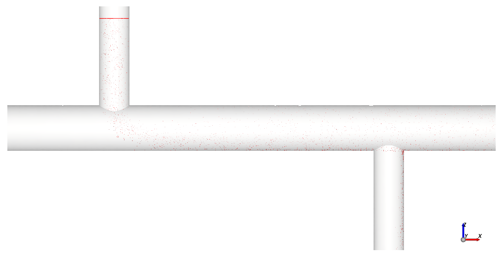
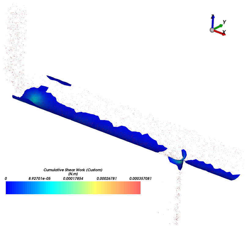
The results are shown below.
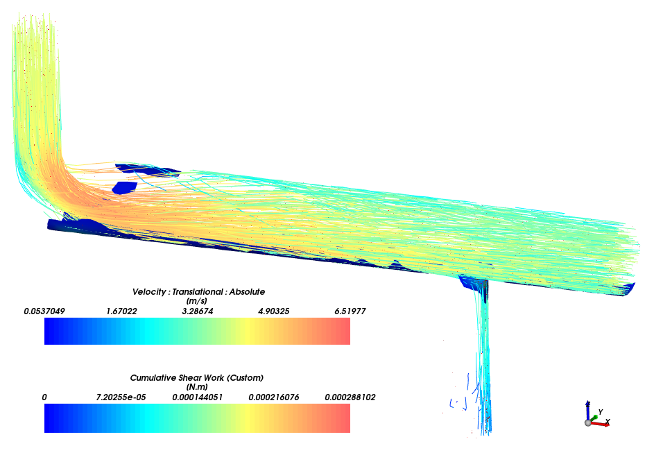
As shown in the images below, most of the shear work happens on the bottom portion of the main pipe.
Of the bottom portion of the main pipe, the regions of highest shear work are:
The region right below the particles' inlet.
The region of the stream separation.
As the shear work is more severe in these regions, they are the most susceptible to wear.
This completes Part B of this tutorial.
Rocky was used to post-process a simulation of a Mixing Tee.
During this tutorial, it was possible to:
Use a Time Plot to identify a steady state for particle flow.
Use Cube and Particles Time Selection User Processes to measure the amount of particle mass that flowed through the outlets.
Analyze the particle size segregation between the outlets by using a Histogram.
Visualize the cumulative shear work on the Mixing Tee geometry by using the Boundary Collision Statistics data that was collected in Part A combined with the Particles Trajectory.
What's Next? If you completed this tutorial successfully, then you are ready to move on to next tutorial.