


(Part A) Set up and process a simulation that makes use of the Liquid Bridge Model external module, which enables you to compute adhesive forces caused by the liquid film that involves the particles when they are wet.
(Part B) Analyze the mixing performance using the Lacey Mixing Index (LMI).
(Part C) Analyze the liquid distribution during the mixing process.
The main purpose of this tutorial is to learn to set up and process a Liquid Bridge simulation for later mixing analysis.
Part B will cover analyzing the mixing performance using the Lacey Mixing Index (LMI) and Part C will cover analyzing the liquid distribution.
The scenario considered in this tutorial is evaluating the mixing performance of a Ribbon Blender combining two different materials: one powder material (dry) and one additive material (wet).
Note: Ribbon Blenders are commonly used in the food, chemical, and pharma industries.
You will learn how to:
Install, enable, and then configure the Liquid Bridge adhesion model
And you will use these features:
Liquid Bridge Model Module
Important: This ADVANCED tutorial contains fewer details, screenshots, and procedures than other Rocky tutorials.
An ADVANCED tutorial is designed for users who are more familiar with the Rocky user interface (UI), and already have a good understanding of the common setup and post-processing tasks.
If you do not already have this level of familiarity, it is recommended that you complete at least Tutorials 01- 05 before beginning this one.
To make use of the referenced external module, you must have Rocky 2025 R2 or later and your version of Rocky must be the same as the SDK version in which the module was compiled.
For this tutorial, an external module will be installed and used.
External modules are not installed with the Rocky product by default; rather, they are downloaded and installed separately.
To install the module, do the following:
Download the ready-to-use module Liquid Bridge Model for your operating system.
Open the folder that downloads and then extract its content.
Copy the 25.2.0 folder you previously extracted to one of the following locations:
Windows: %HOMEPATH% / Documents / Rocky / Modules
Linux: ~/.Rocky / Modules
Restart (or open if already closed) Rocky to refresh the module libraries.

The geometries in this tutorial are composed of:
(1) Tank
(2) Ribbon
These two items will be imported as .stl files, which can be found in the tutorial directory.
To get started setting up this tutorial, do the following:
Download the
dem_tut18_files.zipfile here .Unzip
dem_tut18_files.zipto your working directory.Ensure Rocky 2025 R2 is open.
Create a new project.
Save the empty project to a location of your choosing.
For the Modules step, we will be enabling the Liquid Bridge Model module.
Liquid Bridge Model applies to particles an adhesion model that simulates what happens when a wet particle gets close enough to another particle or boundary for their liquid films to touch or "bridge".
Because the default values already represent water, we will be leaving most of the Liquid Bridge settings as default for this tutorial.

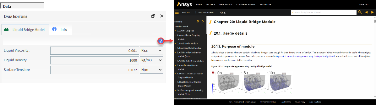
Tip: More information about this module can be found in the Ansys Help by clicking the button as shown.
First, let's turn on the Liquid Bridge Model module:
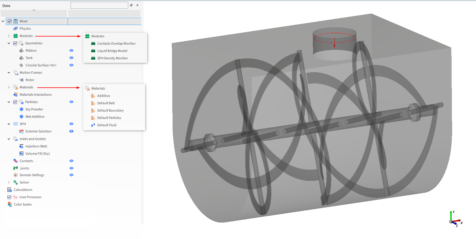
From the Data panel, select Modules.
From the Data Editors panel, enable the Liquid Bridge Model checkbox (as shown).

Tip: If you do not see the Liquid Bridge Model listed here, ensure you have followed the steps on EXTERNAL MODULE.
To see the parameters you are able to set:
From the Data panel, under Modules, select the new Liquid Bridge Model entry.
From the Data Editors panel, view the following parameters:
Liquid Viscosity: Defines the viscosity of the liquid film around particles.
Liquid Density: Defines the density of the liquid film around particles.
Surface Tension: Defines the surface tension of the liquid film around particles.

In addition to those listed in the module itself, additional Liquid Bridge parameters will be available in other locations of the Rocky setup, including:
Materials Interactions
Inlets and Outlets
Note: We will cover these later in the tutorial.
Now that the module is enabled, we can begin setting up other parts of the project.
Use the information in the table that follows to continue setting up the project.
Tip: If you run into settings or procedures in these tables that you are not yet familiar with, please refer to the Rocky User Manual and/or other Tutorials (via the Introductory Tutorials and Advanced Tutorials) to find the detailed instructions you need.
Step Data Entity Editors Location Parameter or Action Settings A Study Study Study Name Mixer B Physics Physics | Momentum Numerical Softening Factor 0.1 [ - ] C Geometries Import Wall Ribbon.stl and Tank.stl with "m" for Import Unit Create Circular Surface D Geometries ﹂Circular Surface <01>
Circular Surface Center Coordinates -0.005, 0.675, 0.315 [m] Max Radius 0.13 [m] E Motion Frames Create Motion Frame F Motion Frames ﹂Frame <01>
Frame Name Rotor Relative Position 0.62, 0, 0 [m] … | Motions Add motion Type Rotation ⯆ Initial Angular Velocity 42, 0, 0 [rev/min] G Geometries ﹂Ribbon
Wall Motion Frame Rotor ⯆ H Materials ﹂Default Boundary
Material Young's Modulus 1e+09 [N/m2] I Materials ﹂Default Particles
Material Bulk Density 593 [kg/m3] Young's Modulus 1e+07 [N/m2] J Materials Create Solid Material K Materials ﹂Material <04>
Material Name Additive Use Bulk Density (Enabled) Bulk Density 640 [kg/m3] Young's Modulus 1e+07 [N/m2] L Materials Interactions … | Default Particles ⯆ Default Particles ⯆
Static Friction 0.2 [ - ] Dynamic Friction 0.2 [ - ] … | Additive ⯆ Additive ⯆
Static Friction 0.2 [ - ] Dynamic Friction 0.2 [ - ] … | Default Particles ⯆ Additive ⯆
Static Friction 0.2 [ - ] Dynamic Friction 0.2 [ - ]
Earlier in the Modules step, we enabled the Liquid Bridge Model module.
Doing so turned on additional parameters in other parts of the Rocky UI, including for Materials Interactions.
The additional Liquid Bridge Model parameters that you can set for your Materials Interactions pairs are as follows:
Bridge Volume Fraction (fb): Defines the fraction of the liquid bridge volume that the particle pair will each contribute to when they are close enough for their liquid films to form a bridge.
Contact Angle (θ): Defines the angle between the surface of the liquid bridge and the particle (and/or boundary) surfaces between which it formed.
Minimum Separation Ratio: Defines the minimum separation ratio between the pair of colliding particles below which the capillary and viscous liquid bridge forces will remain with a constant value. The minimum separation distance (h) is computed as the minimum separation ratio times the biggest particle radius.

Note: For this tutorial, we will be leaving these settings as default.

For this tutorial, we will create one Volumetric Inlet with Dry powder particles and a Particle Inlet with Wet additive particles.
In this way, we will have two distinct layers of particles to better analyze the mixing:
Use the information in the table that follows to continue setting up your simulation:
Step Data Entity Editors Location Parameter or Action Settings A Particles Create Particle B Particles ﹂Particle <01>
Particle Name Dry Powder Particle | Size (1) Size | Cumulative % 0.04 [m] @ 100% C Particles Create Particle D Particles ﹂Particle <01>
Particle Name Wet Additive Material Additive Particle | Size (1) Size | Cumulative % 0.03 [m] @ 100% E Inlets and Outlets Create Particle Inlet F Inlets and Outlets ﹂Particle Inlet <01>
Particle Inlet Name Injection (Wet) Entry Point Circular Surface <01> Particle Inlet | Particles Add row (x1) (1) Particle | Mass Flow Rate Wet Additive ⯆ 72 [t/h] … | Time Stop 1 [s] … | Entry Stop All Injection at Stop Time (Enabled)
Important: The Particle Inlet Mass Flow Rate was set in a way that the Wet Additive mass will be 15% of the total mass (Wet Additive + Dry Powder).
Earlier in the Modules step, we enabled the Liquid Bridge Model module, which turned on additional parameters in other parts of the Rocky UI, including for Inlets and Outlets.
This additional parameter appears on a new Modules sub-tab for your Inputs:
Liquid Mass: Defines the liquid mass that will be applied to each particle within the selected Particle set.
Note: The Particle set listed here is defined on the Particles sub-tab.
From the Modules sub-tab, define Liquid Mass.

Now, we'll create a Volumetric Inlet that injects the Dry Powder particles, and will finish setting up the rest of our project.
Note: We want the Dry Powder particles to be completely dry at the time of injection, so we will leave the Liquid Mass setting as 0 (zero).
Use the information in the table that follows to finish setting up your project.
Step Data Entity Editors Location Parameter or Action Settings A Inlets and Outlets Create Volumetric Inlet B Inlets and Outlets ﹂Volumetric Inlet <01>
Volumetric Inlet Name Volumetric Fill (Dry) Volumetric Inlet | Particles Add row (x1) (1) Particle | Mass Dry Powder ⯆ 113 [kg] Volumetric Inlet | Region Seed Coordinates 0, -0.375, 0 [m] Geometries | Ribbon (Enabled) Geometries | Tank (Enabled) Box bounds | Center Coordinates 0, -0.414, 0 [m] Box bounds | Dimensions 1.6, 0.296, 1.1 [m] C Solver Solver | Time Simulation Duration 10 [s] Solver | General Simulation Target CPU ⯆
With a 3D View window opened, your Data panel and Workspace should look similar to the below image.
From the Solver entity, click Start.
The Simulation Summary screen appears (as shown), then processing begins.
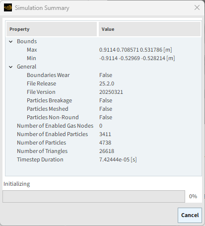

Tip: You can use the Auto Refresh checkbox to view in a 3D View window the results during processing.
This completes Part A of this tutorial, in which Rocky was used to set up and process a Ribbon Blender simulation.
During this tutorial, it was possible to:
Download, install, enable, and set up the Liquid Bridge Model module.
Define new Materials and configure their module-specific Materials Interactions.
Create multiple Inputs, and define module-specific parameters within them.
What's Next? If you completed this tutorial successfully, then you are ready to move on to Part B and/or Part C and post-process this project.
The main purpose of this tutorial is to use the results of the simulation we set up and processed in Part A to analyze the mixing efficiency using the Lacey Mixing Index (LMI).
As a reminder, the scenario considered in this tutorial is a Ribbon Blender mixing two different materials: one (dry) powder material and one (wet) additive material.
You will calculate the LMI by learning how to:
Tag particles with a certain defined criteria
Use Cylinder and Eulerian Statistics User Processes to define discrete cells
Calculate properties statistics and Custom Properties using mathematical expressions
Build property filters by using the Filter User Process
Calculate custom properties from other properties in a Time Plot
And you will use these features:
Tagging Particle Calculations
User Processes, including:
Cylinder
Eulerian Statistics
Filter
Time Plots (including the Add Formula feature)
Important: Important: This ADVANCED tutorial contains fewer details, screenshots, and procedures than other Rocky tutorials.
An ADVANCED tutorial is designed for users who are more familiar with the Rocky user interface (UI), and already have a good understanding of the common setup and post-processing tasks.
If you do not already have this level of familiarity, it is recommended that you complete at least Tutorials 01- 05 before beginning this one.
To make use of the external module referenced, you must have Rocky 2025 R2 or later and your version of Rocky must be the same as the SDK version in which the module was compiled.
Tip: If you are unsure which version of Rocky you have, check the Rocky About screen. (From the Help menu, click About, and then view the Version information).
If you completed Part A of this tutorial, ensure that Rocky project is open. (Part B will continue from where Part A left off.)
If you did not complete Part A, do all of the following:
Download the
dem_tut18_files.zipfile here .Unzip
dem_tut18_files.zipto your working directory.Open Rocky 2025 R2.
Important: To make use of the Rocky project file provided, you must have Rocky 2025 R2. If you have an earlier version of Rocky, please upgrade Rocky to version Rocky 2025 R2, or complete Part A from scratch.
From the Rocky program, click the Open Project button, find the dem_tut18_files folder, then from the tutorial_18_A_pre-processing folder, open the tutorial_18_A_pre-processing.rocky file.
Process the simulation. (From the Data panel, select Solver and then from the Data Editors panel, click the Start button.)
With the processing complete, we can now start analyzing our results.
At any given time, Properties can be used to color the Particles in a 3D View window.
For example, you can do the following:
From the Particles entity, on the Properties tab, right-click Particle Group, point to 3D View and then click Show in new 3D View.
Tip: You might need to make the Tank geometry transparent (or hidden) to see the particles.

In order to evaluate the uniformity of mixing, we will divide the mixture into samples and will measure the Mass Fraction of Additive Particles in each sample.
A good degree of mixing means that the mass fractions of the samples are approximately the same.
Each discrete volume (cell) will represent a different sample of our mixture.

To compare the degree of uniformity between samples, we can calculate their Additive Mass Fraction Variance.
The higher the variance, the more heterogeneous is the system, which means a poor degree of mixing.
The Lacey Mixing Index (LMI) is often used to evaluate the uniformity of mixing. It can be interpreted as a normalization of the mass fraction variance, and will provide values ranging from 0 to 1.
An index of 0 (zero) means that the mass fraction variance is the maximum theoretical value and also means complete segregation (no mixing achieved).
An index of 1.0 means that the mass fraction variance is the minimum theoretical value and also means a completely random mixing (maximum mixing achieved).
A "good" mixture can be defined as achieving an index between 0.75 - 1.0.
The Lacey Mixing Index can be defined as:
 | (18–1) |
The equation components are described below.


Where:
 : Number of cells (Eulerian Statistics Divisions)
  : Average Additive Mass fraction across cells
  : Additive Mass fraction of the whole system
  : Additive Mass fraction in the cell i
  : Average number of particles across cells
  : Additive Mass in the cell i
  : Main Product Mass in the cell i
Particles Properties and Tagging Calculations will be used to filter the Wet Additive Particles.
Tagging allows you to define a Global value to particles that meet a specific criterion in a particular Output Time.
To select a group of particles, we will create a new Filter User Process that filters particles based on their properties.
Filter the Particles by the Wet Additive Particle Group by using the information in the table below:
Step Data Entity Editors Location Parameter or Action Settings A Particles Create a Filter User Process B User Processes ﹂Filter <01>
Filter Name Wet Additive Propertie Particle Group ⯆ Cut Value 1 [<ind>] To see only the filtered particles, use the eye icons on the Data panel to hide the main Particles entity and make the Wet Additive User Process visible.

In this tutorial, we will Tag the Wet Additive Particles with a value of 1, which will automatically make all other untagged particle groups have a value of 0.
This separation will be needed later when we calculate the mass of the Wet Additive particles only.
Tag the Wet Additive particles using the information in the table below:
Step Data Entity Editors Location Parameter or Action Settings A Particles Create a Tagging calculation over the Wet Additive entity B Calculations ﹂Tagging (Wet Additive)
{t=0[s], v=1}
Tagging Time Range Filter | Domain Range Specific Time ⯆ Time Range Filter | At time 1 [s] Tag Value 1 [s]
Next, we will define a new property that multiplies the Tag value and the Particles Mass value, which we will call Mass If Additive.
In this way, if the particle is a Wet Additive particle, the value of this new custom property is the Particle Mass. Otherwise, the value will be zero.
Create a new Custom Property using the information in the table below:
Step Item Location Parameter or Action Settings A Particles Properties Add new custom property (button) B Add new (dialog box) Name Mass if Additive Output unit kg Inputs | Particle Mass (Enabled) Inputs | Tagging (Wet Additive)... (Enabled) C Custom Property (dialog box) Expression A*B
A new property called Mass If Additive (Custom) appears on the Properties tab for Particles.
Now that we've defined the Mass If Additive property, we need to divide the Ribbon Blender tank into samples.
For this step, we will create a Cylinder User Process and then apply Eulerian Statistics divisions to the cylinder.
The Additive Mass Fraction will then be calculated for each individual cell by adding a new expression defined as the Additive Mass divided by the Particle Mass.

Use the information in the table that follows to set up the processes.
Step Data Entity Editors Location Parameter or Action Settings A Particles Create a Cylinder User Process B User Processes ﹂Cylinder <01>
Cylinder Size 1.1, 1.5, 1.1 [m] Center 0, 0, 0 [m] Orientation | Method Angles ⯆ Orientation | Rotation 0, 0, 90 [dega] C User Processes ﹂Cylinder <01>
Create a Eulerian Statistics User Process D User Processes ﹂Eulerian Statistics <01>
Eulerian Statistics Radial Divisions 1 [ - ] Tangential Divisions 18 [ - ] Axial Divisions 8 [ - ]
Next, we will calculate the Additive Mass Fraction in each cell.
First we need to calculate both the sum of all particles mass and the Wet Additive particle mass in each cell.
Use the information in the table that follows to add two new Eulerian properties:
Step Item Location Parameter or Action Settings A User Processes ﹂Eulerian Statistics <01>
Properties Add and edit properties for source entity (button) B Add or edit eulerian properties Add a new property C Add new property (dialog box) Operation Sum ⯆ Particle Property Mass If Additive (Custom) ⯆ Add Property Operation Sum ⯆ Particle Property Particle Mass ⯆ Add Property
From the Properties tab of the Eulerian Statistics <01> entity, the two new custom properties appear.
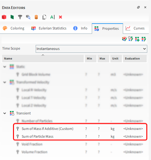
The last step to visualize the mass fraction is to divide the Sum of Mass If Additive (Custom) by the Sum of Particle Mass using a new Custom Property.
Use the information in the table that follows to create this new custom property.
Step Item Location Parameter or Action Settings A User Processes ﹂Eulerian Statistics <01>
Properties Add new custom property (button) B Add new (dialog box) Name Additive Mass Fraction Output unit - Inputs | Sum of Mass If Additive (Enabled) Inputs | Sum of Particle Mass (Enabled) C Custom Property (dialog box) Expression A/B Note: For Step C, ensure the expression you enter represents Sum of Mass If Additive (Custom) divided by Sum of Particle Mass.
The newly created property will be available on the Properties tab for the Eulerian Statistics <01> entity.
Drag and drop the new Additive Mass Fraction (Custom) property onto a 3D View window.
By using the slider on the Time toolbar, you can see how the Mass Fraction is distributed in the cells over time.

In order to evaluate the Lacey Mixing Index (LMI) unbiased, we'll select and analyze only those cells with the highest amounts of particles, to ensure better representative samples.
For this step, we will filter the cells based on their mass.
Use the information in the table that follows to create a property process to filter those cells:
Step Data Entity Editors Location Parameter or Action Settings A User Processes ﹂Eulerian Statistics <01>
Create a Filter User Process B User Processes ﹂Filter <01>
Filter Name Sample LMI Property Sum of Particle Mass ⯆ Mode Select ⯆ Type Range ⯆ Minimum value 1 [kg] Maximum value 10 [kg]
Important:
Modifying the number of Eulerian Statistics divisions changes the total particle Mass in each sample. Therefore, the mass range used to filter the samples through the Filter Process would be different.
The range of Sum of Particle Mass defined through the Property Process above should be adjusted based on the Property limits.
Tip: You can view the limits by clicking the Load Limits button on the Property tab when defining a Filter User Process.
The number of Eulerian Statistics cells (volume of samples) affect the calculated value of Lacey Mixing Index. For example, a higher number of divisions would increase the heterogeneity between samples and, therefore, their variance.
A sensitivity analysis should be performed to find the optimum number of cells. For example, coarser particles would require a greater volume of each sample (so, the particles wouldn't be bigger than a cell), reducing the number of cells.
From the Sample LMI entity, on the Properties tab, right-click Additive Mass Fraction (Custom), point to Time Plot, point to Show in new Time Plot, and then click Variance. (Resulting plot shown.)

The plot represents
 , Additive Mass Fraction Variance,
represented by:
, Additive Mass Fraction Variance,
represented by: 
(18–6)
Where
is the number of cells, is the Additive Mass Fraction in the
cell i and is the Additive Mass Fraction Average
(taken across Eulerian Statistics cells). From the Sample LMI entity, on the Properties tab, right-click Number of Particles, point to Time Plot, point to Show in selected Time Plot, and then click Average. (Resulting plot shown.)

If we recall from the setup in Part A, the System Additive Mass Fraction (
) is 15%. So next, we need to define
 and
and  (see equations below) using the Add
Formula feature in the Time Plot window we
already created.
(see equations below) using the Add
Formula feature in the Time Plot window we
already created.Use the information in the table that follows to create formulas in the Time Plot:
Step Location Parameter or Action Settings A Time Plot | Table Add Formula B Add Expression Curve Caption Fully Unmixed Curve Expression 0.15*(1-0.15) C Time Plot | Table Add Formula D Add Expression Curve Caption Fully Mixed Curve Expression E1/C E Time Plot | Table Add Formula F Add Expression Curve Caption LMI Curve Expression (B-E1)/(E2-E1) Note: Make sure that the B column represents the Variance: Additive Mass Fraction (Custom) calculation, the C column represents the Average: Number of Particles (Mixer - Sample LMI), the E1 column represents the Fully Unmixed calculation and the E2 column represents the Fully Mixed calculation.
If you switch to the Plot tab, you can now see how the Lacey Mixing Index (orange dashed line) changes over time.

Tip: Change the Axes Layout to By Quantity to facilitate visualization.
We can see that the LMI reaches 0.99 (which we can consider "fully mixed") at 6.8s.
Note: Your results might differ from the ones shown in this tutorial.
Tip: Press and hold the Shift key and then left-click the curves with your mouse to see specific values.

It is also possible to see this result from the Table tab.


This completes Part B of this tutorial, in which Rocky was used to calculate the Lacey Mixing Index (LMI) of the Ribbon Blender simulation we set up and processed in Part A.
During this tutorial, it was possible to:
Use Tagging Particle Calculations to mark particles with a certain defined criteria.
Use a Cylinder User Process to define an Eulerian Statistics User Process in order to calculate properties statistics in discrete cells.
Calculate Custom Properties using mathematical expressions.
Build property filters using the Filter User Process.
Calculate custom curves from other curves in a Time Plot.
What's Next? If you completed this tutorial successfully, then you are ready to move on to Part C and continue post-processing this tutorial.
The main purpose of this tutorial is to use the results of the liquid bridge simulation we set up and processed in Part A to analyze the distribution of liquid during mixing.
As a reminder, the scenario considered in this tutorial is a Ribbon Blender mixing two different materials: one (dry) powder material and one (wet) additive material.
You will learn how to:
Display liquid mass in a 3D View window
Change the color-scale of a 3D View window
Use a Filter User Processes to analyze liquid distribution and dispersion
And you will use these features:
Liquid Mass Property
User Processes, including:
Property
Time Plots
Histograms
Important: Important: This ADVANCED tutorial contains fewer details, screenshots, and procedures than other Rocky tutorials.
An ADVANCED tutorial is designed for users who are more familiar with the Rocky user interface (UI), and already have a good understanding of the common setup and post-processing tasks.
If you do not already have this level of familiarity, it is recommended that you complete at least Tutorials 01- 05 before beginning this one.
To make use of the external module referenced, you must have Rocky 2025 R2 or later and your version of Rocky must be the same as the SDK version in which the module was compiled.
Tip: If you are unsure which version of Rocky you have, check the Rocky About screen. (From the Help menu, click About, and then view the Version information).
If you completed Part A (and/or ) of this tutorial, ensure that Rocky project is open. (Part C will continue from where Part A (or Part B) left off.)
If you did not complete Part A (and/or Part B), do all of the following:
Download the
dem_tut18_files.zipfile here .Unzip
dem_tut18_files.zipto your working directory.Open Rocky 2025 R2.
Important: To make use of the Rocky project file provided, you must have Rocky 2025 R2. If you have an earlier version of Rocky, please upgrade Rocky to version Rocky 2025 R2, or complete Part A from scratch.
From the Rocky program, click the Open Project button, find the dem_tut18_files folder, then from the tutorial_18_A_pre-processing folder, open the tutorial_18_A_pre-processing.rocky file.
Process the simulation. (From the Data panel, select Solver and then from the Data Editors panel, click the Start button.)
With the processing complete, we can now start analyzing our results.
Earlier in Part A we enabled the Liquid Bridge adhesion model, which performs the following functions during processing:
(1) Tracks liquid content in each particle
(2) Calculates capillary and viscous forces
(3) After particles separate (bridge ruptures), redistributes liquid

After processing the simulation, a new property is available for Particles:
Liquid Mass: Provides the mass of the liquid film around each individual particle.
Important: The liquid mass is not included in the particle mass. For example, if the dry particle has 0.1 kg and you add 0.1kg of liquid, the particle mass will remain 0.1 kg.
We can use this new property to see how the dry particles were affected by the wet particles during mixing.
From the Particles entity, on the Properties tab, right-click Liquid Mass, point to 3D View and then click Show in new 3D View.
Make the Tank and Ribbon geometries transparent (or hidden) to see the particles.

The Liquid Mass of the particles is shown.
To change the color scale, do the following:
Right-click the color scale, and then select Edit.

From the Data Editors panel, click the ... button next to Color-scale.
From the Color-scale dialog, click the ... button again, and then select the red-to-blue color scale (as shown).

Below the red-to-blue Color-scale, double-click the red-colored dot and then from the Select Color dialog, select the white color (as shown), and then click OK.

The Color-scale should now show white-to-blue.
Click OK to close the dialog.
From the Data Editors panel, under Limits, define Limit options, and then define the Limits values (as shown).

Use the slider on the Time toolbar to see how the liquid from the Wet Additive (blue) is transferred to the Dry Powder (white) over time.

We can also plot the average Liquid Mass of both the dry and wet particles on a Time Plot.
But first, we need to separate the groups by creating two Filter User Processes.
Filter the Particles by Particle Group by using the information in the following table.
Note: If you completed Part B of this tutorial, you can skip steps A and B since you already have the Wet Additive Filter User Process.
Step Data Entity Editors Location Parameter or Action Settings A Particles Create a Filter User Process B User Processes ﹂Filter <01>
Filter Name Wet Additive Property Particle Group ⯆ Type Value ⯆ Cut Value 1 [<ind>] C Particles Create a Filter User Process D User Processes ﹂Filter <01>
Filter Name Dry Powder Property Particle Group ⯆ Type Value ⯆ Cut Value 0 [<ind>] From the Data panel, under User Processes, multi-select both the Dry Powder and Wet Additive items.
From the Data Editors panel, on the Properties tab, right-click Liquid Mass, point to Time Plot, point to Show in new Time Plot, then click Average.
The resulting Time Plot shows that by the end of the simulation, the liquid that was initially only in the wet particles is after mixing, evenly distributed throughout both the wet and dry particles.

Now let's analyze the liquid dispersion, starting from the beginning of the simulation.
From the Time toolbar, move the slider back to [20] 1 s.
From the Data panel, under User Processes, multi-select both the Dry Powder and Wet Additive items.
From the Data Editors panel, on the Properties tab, right-click Liquid Mass, point to Histogram, and then click Show in new Histogram.

Use the information in the table that follows to configure the histogram:
Step Item Parameter or Action Settings A Histogram (window) Configure histogram (button) B Configure Histogram (dialog box) Number of Bins 20 [ - ] Percent Values (Enabled) Properties | Liquid Mass (Selected) Limits User Defined ⯆ Min 0 [kg] Max 0.02 [kg]
The resulting Histogram (at 1 s) shows that at the very beginning of the simulation, 100% of the liquid is concentrated on the wet additive.

You can explore how the liquid spreads over time by moving the Time slider forward.
For example, a few seconds into the simulation, fewer particles remain completely dry than at the beginning of the simulation. (Results shown at 3 s.)

By the end of the simulation, the liquid content is gathering around the average. (Results shown at 10 s.)

This completes Part C of this tutorial, in which Rocky was used to analyze the liquid distribution within the Ribbon Blender simulation we set up and processed in Part A.
During this tutorial, it was possible to:
Understand the results of a Liquid Bridge simulation
Display the Liquid Mass property in a 3D View window
Change the colors and limits of a 3D View's Color-scale
Use Filter User Processes and a Time Plot to analyze liquid distribution
Use Filter User Processes and a Histogram to analyze liquid dispersion
What's Next? If you completed this tutorial successfully, then you are ready to move on to next tutorial.