


(Part A) Learn how to set up and process a simulation that modifies the surface of geometries to show the effects of wear.
(Part B) Learn how to visualize the wear modification to the surface of the geometry, add particle trajectories, and analyze properties derived from contacts.
(Part C) Learn how to analyze the energy balance of the system by using particle energies and particle energy spectra data.
The main purposes of this tutorial are to:
Learn how to set up and process a simulation that modifies the surface of geometries to show the effects of wear (Parts A and B).
Learn how to analyze the energy balance of the system (Part C).
The scenario considered is that of a semi-autogenous grinding (SAG) mill, which is a rotating machine that contains steel balls and ore.
SAG mills are used in the mining industry to grind ore particles into smaller pieces. To save processing time, only a slice of the mill will be simulated.
You will learn how to:
Collect collision statistics, particle energies, and energy spectra data
Define a rotation motion
Model surface wear, and properly mesh geometries
Add a custom Material type
Define a Volumetric Inlet for particles
Turn on the collection of Contacts data
Define periodic domains
And you will use these features:
Modules
Motion Frames
Surface Wear Modification Model
Cartesian Periodic Domains
This tutorial assumes that you are already familiar with the Rocky user interface (UI) and with the project workflow.
If this is not the case, please refer to Tutorial 01 – Transfer Chute for a basic introduction about Rocky usage before beginning this tutorial.
Tip: If you are unsure which version of Rocky you have, ask your IT department, or contact Rocky Support for assistance.
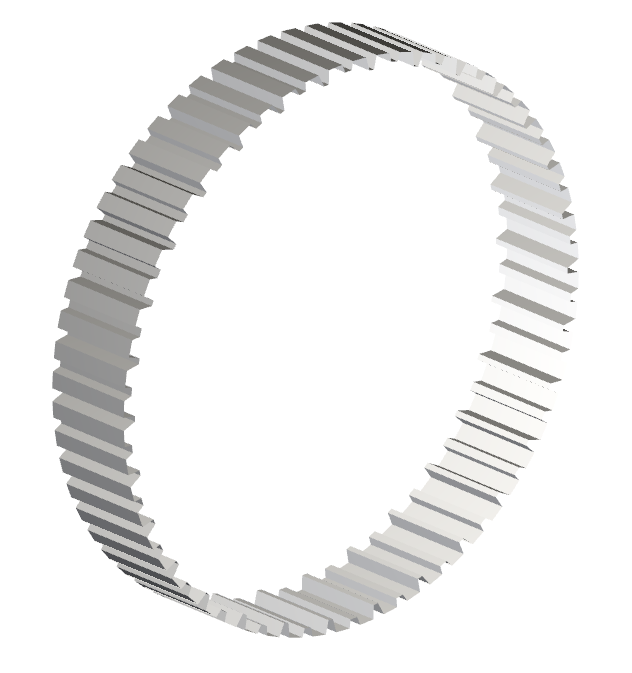
The geometry in this tutorial is composed of:
Mill slice
In the tutorial directory the .stl file can be found.
To start the tutorial, you have to create a new project:
Download the
dem_tut04_files.zipfile here .Unzip
dem_tut04_files.zipto your working directory.Open Rocky 2025 R2. (Look for Rocky 2025 R2 in the Program Menu or use the desktop shortcut.)
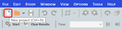
From the Rocky program, click the New Project button, or from the File menu, click New Project (Ctrl+N).
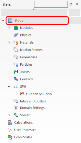
The Study entity covers the first step of the simulation setup. The purpose is to define any useful information for the project.
From the Data panel, click Study 01.
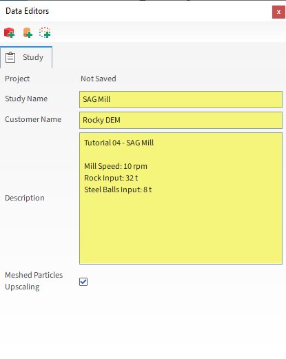
From the Data Editors panel, enter the project information.
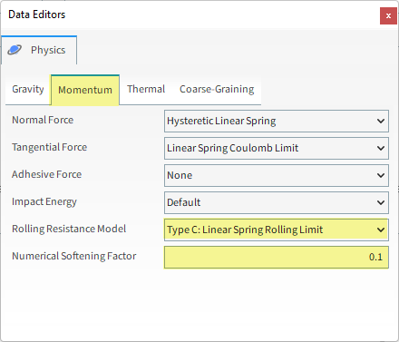
For the Physics step, we will be lowering the softening factor to reduce simulation time, and will also set a rolling resistance model.
Important: Lowering the softening factor may cause excessive overlaps between particles and between particles and boundaries.
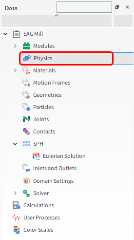
From the Data panel, select Physics.
From the Data Editors panel, select the Momentum sub-tab, and then set the Rolling Resistance Model and change the Numerical Softening Factor.
For the Modules step, we will be turning on the collection of some additional data.
But before we take these steps, it is necessary to understand more about Modules:
In Rocky, Modules refer to separate pieces of code that add in discrete features or functionality within your project.
By having the state of (most of) these Modules be off by default, calculations that you may not require are avoided, which saves processing time and reduces file size.
But it also means that if you want to use of a Module, you must remember to turn it on during your simulation setup.
In addition, some Modules add new options within other parts of the Rocky setup so it is important that you turn on your Modules before setting up the rest of your project.
It is also important to understand that some Module settings will override similar default settings in the Rocky UI.
Tip: To find out what models or settings are affected by a Module, you can view the Affected Simulation Entities information on the Module's Info tab.
There are several Modules provided by default in Rocky. (Listed on next slides.)
You may also have access to other custom Modules that are not included with Rocky by default.
Custom Modules are installed via zip file from the Ready-to-use Modules page.
After installation, they will appear in Rocky on the Data Editors panel for Modules.
Tip: You can make your own custom Modules by using Rocky's Solver SDK functionality. (See the Rocky Solver SDK Manual and the Tutorial 23 for details.)
When working with Modules, it is important to realize that:
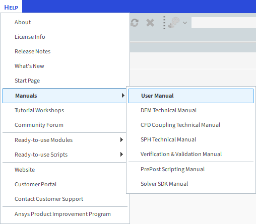
Default Modules are defined in the User and Technical Manuals, which can be found from the Rocky Help | Manuals menu.
Custom Modules have their own documentation that can be found in the Rocky Module Manual.
The following sixteen Modules are available by default in Rocky:
Boundary Collision Statistics: Enables the collection of boundary-related collision (with particles) data, such as collision frequency, intensities, and impact velocities.
Note: We will enable this module within this tutorial.
CFD Coupling Particle Statistics: Enables the collection of particle-fluid interactions, such as drag, lift, and virtual mass forces.
Contacts Energy Spectra: Enables the collection of collision-based energy values during the simulation and the resulting data is categorized by the contact pair (particle group and/or geometry).
Note: We will enable this module within this tutorial.
Contacts Overlap Monitor: Checks each contact pair (particle-particle or particle-boundary) for the amount that they overlapped the percentage of which is determined by the size of the smallest particle in the contact pair and raises a message in the Simulation Log panel if an overlap exceeds any of the three warning levels you define.
Note: By default, this module is always enabled.
Inter-group Collision Statistics: Enables the collection of energy dissipation data for each particle-particle and particle-boundary pair.
Note: We will enable this module within this tutorial.
Inter-particle Collision Statistics: Enables the collection of particle-related collision data between all particles in the simulation.
Note: We will enable this module within this tutorial.
Intra-particle Collision Statistics: Enables the particle-related collision data affecting the surfaces of a particular particle set.
Joint Statistics: Enables the collection of data for Joints when present in the simulation.
Multibody Dynamics FMU Coupling: Enables the coupling between Ansys Rocky and Ansys Motion software.
Particle Instantaneous Energies: Enables the calculation of the kinetic and potential energies of each individual particle in the simulation.
Note: We will enable this module within this tutorial.
Particles Energy Spectra: Enables the collection of energy values during the simulation that are related only to particles, and the resulting data is classified by size and particle group.
Note: We will enable this module within this tutorial.
SPH Boundary Interaction Statistics: Enables the collection of boundary-related collision (with fluid) data, such as forces, torque and power.
SPH Density Monitor: Monitors the density values associated to the SPH elements during a simulation and issues possible related warnings.
Note: By default, this module is always enabled.
SPH HTC Calculator: Enables the estimation of heat transfer coefficient.
SPH Mass Flow Rate: Enables the measure of fluid flow rate through a surface.
SPH-DEM Interaction Statistics: Enables the collection of fluid-particle interaction data, such as forces, torque and heat transfer.
To enable the modules for this tutorial, do the following:
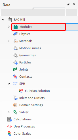
From the Data panel, select Modules.
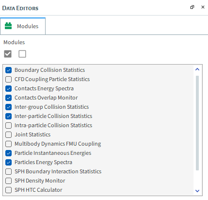
From the Data Editors panel, under Modules enable the following checkboxes:
For this tutorial, we are primarily interested in the power- and energy-related data that will be collected by these Modules.
To save processing power and space, we can limit our collections to only the kinds of data we need.
Note: This applies only to the five Collision Statistics and Energy Spectra modules we enabled; it is not possible to limit the data collection for Particle Instantaneous Energies.
Let's start by defining what data we want for Boundary Collision Statistics:
From the Data panel, under Modules, select Boundary Collision Statistics.
From the Data Editors panel, enable the Intensities checkbox (as shown).
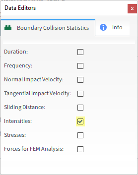
Note: With Intensities enabled, Rocky will collect the average dissipation and impact power values measured by each individual geometry triangle. This can be useful for analyzing impact wear or power draw.
Continue with the remaining two statistics modules:
From the Data panel, under Modules, select Inter-group Collision Statistics.
From the Data Editors panel, enable the Energy Dissipation checkbox (as shown).
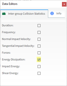
Note: With Energy Dissipation enabled, Rocky will collect the energy dissipation values of the collisions recorded for each particle-particle and particle-boundary pair in the simulation.
From the Data panel, under Modules, select Inter-particle Collision Statistics.
From the Data Editors panel, enable the Power checkbox (as shown).
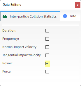
Note: With Power enabled, Rocky will collect the dissipation, impact and shear power values resulting from the collisions recorded for each individual whole particle or fragment, during an output timestep.
In Rocky, you can use a Breakage Model to simulate the breakage behavior of your particles. For our SAG Mill case, this would be useful information to analyze.
However, breakage models can increase both the computational cost and the processing length of your simulation.
With this in mind, Rocky offers a less costly and faster way to analyze breakage called Energy Spectra, which has the following features:
Collects energy statistics based upon the following two gathering methods:
Particle based: Energy is gathered per particle type and size.
Contact based: Energy is gathered per contact pair (particle and/or geometry) and size.
Enables you to limit your data collection in the following ways:
By the type of energy you want to collect: Dissipation, Impact, and/or Shear.
By the particle groups and/or geometries you want to participate in the collection.
Collecting these kinds of energy statistics can help with the prediction of breakage and attrition rates for continuous processes such as grinding mills.
In Rocky, energy spectra is defined via two separate modules.
For each module, you can set the following:
What type of Energy collection you want.
Number of Bins: Defines the resolution of the resulting energy curves. The higher the number of bins, the better the resolution.
Minimum and Maximum Energy (or Specific Energy): Defines the left and right limits of the resulting Curves Energy (or Specific Energy) axis.
Start Time and Time Delay After Release: Defines at what point in the simulation the data is collected.
After defining the parameter on the module itself, there are module-specific parameters enabled on the particle group and/or geometries involved in the simulation.
These additional parameters define the entity as participating in the energy spectra collection or not.
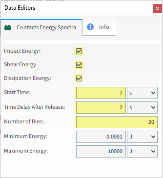
Let's continue to set up our modules by defining Contacts Energy Spectra:
From the Data panel, under Modules, select Contacts Energy Spectra.
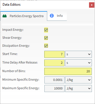
From the Data Editors panel, enable all three Energy checkboxes (as shown), and then define all of the following (as shown):
Start Time
Time Delay After Release
Number of Bins
Repeat similar steps for the Particles Energy Spectra module:
From the Data panel, under Modules, select Particles Energy Spectra.
From the Data Editors panel, enable all three Energy checkboxes (as shown), and then define all of the following (as shown):
Start Time
Time Delay After Release
Number Of Bins
Both of the Energy Spectra modules and the Inter-group Collisions Statistics module enable additional parameters in other parts of the UI.
For each item listed below, you can determine whether it will participate in the type of collection specified:
Each wall component.
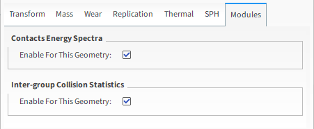
Each particle group.
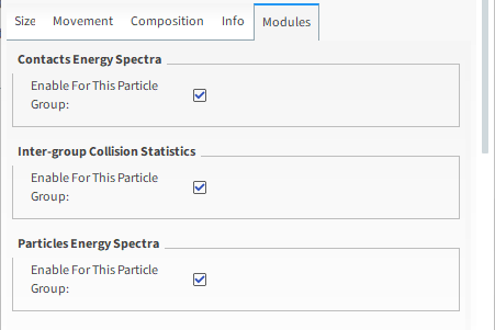
Note: Geometry and particle group setup will be covered later in this tutorial. However, as these module-specific settings are all enabled by default, we will leave them as-is for this tutorial, unless specified.
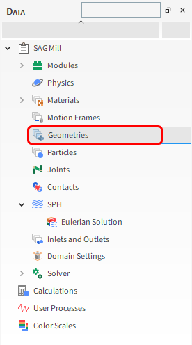
For the Geometries step, we will import the geometry file in .stl format:
From the Data panel, right-click Geometries and then click Import Wall.
From the Select file to import dialog, navigate to the dem_tut04_files folder that you previously downloaded, find the geometry folder, and then select the following file:
Mill.stl
Click Open.
(Save your project now if you have not already done so.)
From the Import File Info dialog, select "mm" as Import Unit, ensure that the option Convert Y and Z axes is cleared (unchecked), and then click OK.
After the geometry is imported, you can view the results in a 3D View window:
Clicking and drag the Geometries entity from the Data panel to the Workspace. A new 3D View window appears showing the geometries that you imported.
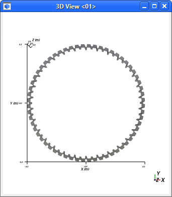
Tip: Because this geometry is aligned with the global Z-direction (no surfaces on the XY plane), it can be hard to see in the 3D View window if your projection is set to Orthogonal instead of perspective.
Change the projection shown in the 3D View window by doing the following:
Select the 3D View window.
From the Camera Visualization toolbar, click the Change projection:Default/Orthogonal button until it shows the Default (perspective) projection.

Your geometry should appear clearly now.
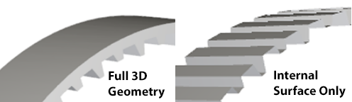
You may notice that we have imported only the internal surface of the 3D geometry.
This method is a best practice for mill slice simulations where you are also calculating surface wear modification.
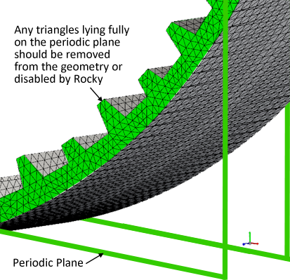
Doing so helps you avoid any potential wear issues that can occur to triangles (shown in green) that are parallel and coincident to the plane used by the periodic domain.
Important: If you do choose to include these triangles, Rocky will disable them by default. However, this disabling can itself lead to other wear calculation instabilities. Therefore, it is best to just avoid including these triangles in the first place.
For the Motion Frames step, we will create two separate Rotation motions within the same Frame, and will then apply this Motion Frame to the mill slice geometry.
The two separate motions represent the following actions:
Mill start: This includes 3 s of constant Angular Acceleration.
Steady state rotation: Starting from 3 s onward, a constant Angular Velocity will be applied, which allows the mill to reach a steady state by 5 s.
When the motion Type of Rotation is selected, the following options are available:
Initial Angular Velocity: The angular velocity at the Start Time.
Angular Acceleration: The rate of change of the angular velocity.
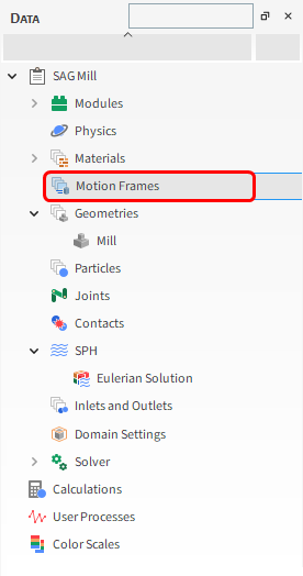
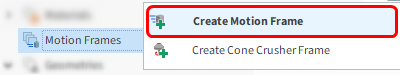
To add a new Motion Frame, do the following:
From the Data panel, right-click Motion Frames and then select Create Motion Frame.
From the Data panel, under Motion Frames, select the newly added Frame <01> entry.
From the Data Editors panel, on the Frame tab, define the parameters as shown next.
To define the first motion frame:
Set the Name: Rotation Motion.
To create a new motion using this Frame, click the green plus button (Add motion).
Define the Stop Time, Type and Angular Acceleration (and units).
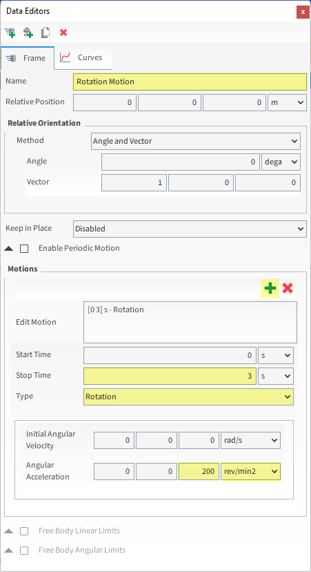
Tip: Because Rocky will automatically translate an entered value based upon the unit you select, it is best to select the unit first before you enter the value.
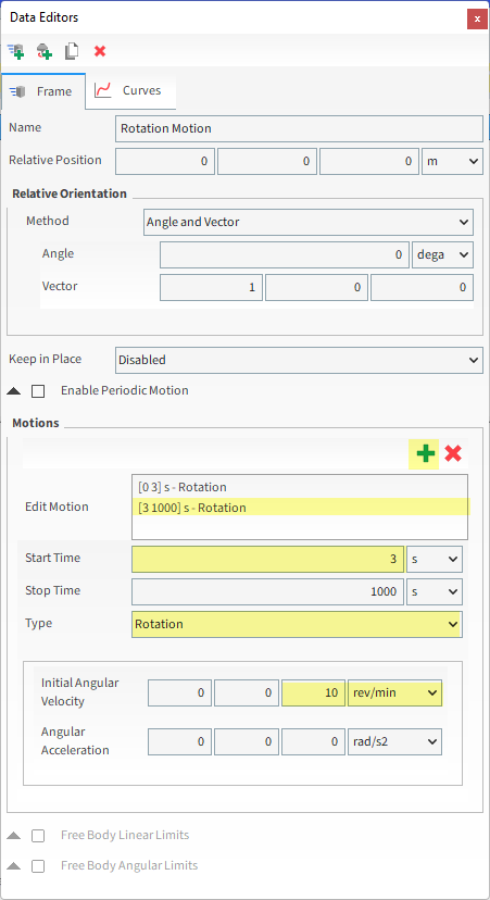
Now let's create a second motion within the same Frame:
Click the green plus button (Add motion) once more.
Define Start Time, Type and Initial Angular Velocity (and units).
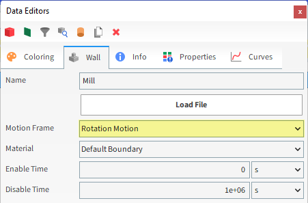
Once the Motion Frame has been created, it must be assigned to the geometry.
From the Data panel under Geometries, select Mill.
From the Data Editors panel, on the Wall tab, select Rotation Motion from the Motion Frame drop-down list (as shown).
For this tutorial, since the geometry has a motion with displacement assigned, the movement can be previewed using the Motion Preview window.
From the Data panel, select Motion Frames.
From the Data Editors panel, click Preview. A new window will appear showing the geometry and the created Frame.
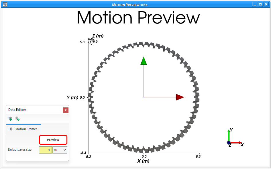
Tip: To better see the frame axes, change the Default axes size parameter (as shown).
The Time toolbar can be used to play the preview. The yellow color of the slider indicates that the simulation has not yet been processed.
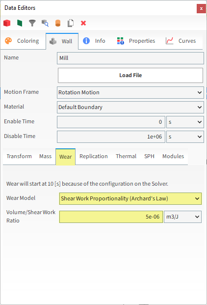
For this tutorial, we will activate the Shear Work Proportionality (Archard's Law) wear model on the Mill slice.
This will enable us to visually evaluate the changes to the surface of the geometry due to the predicted particle contact.
To enable this model, do all of the following:
From the Data panel, under Geometries, select the Mill component.
From the Data Editors panel, select the Wall | Wear tab, and then define both the Wear Model and Volume/Shear Work Ratio options.
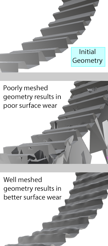
When analyzing wear, it is very important to set the geometry parameters correctly, especially the Triangle Size option.
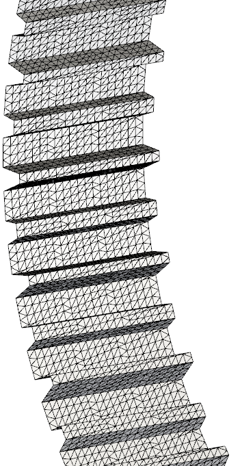
The number of triangles defines how refined the mesh will be when computing wear (and other geometry results).
Tips for proper meshing:
Keep the mesh refined enough to analyze the wear but not so fine that it excessively increases the computational time.
Avoid very fine triangles near the lifter tips as this can make the wear unstable.
To help avoid instabilities, consider doing the following in your CAD program before you import geometries into Rocky:
Remove small details and curvatures.
Fill in any small gaps between components. (For example, make use of the Shrinkwrap feature in Ansys Discovery).
You may also want to mesh your geometries in a program outside of Rocky, and then import the results.
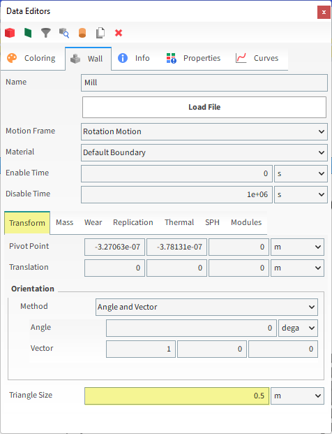
For this tutorial, we will decrease the triangle size in Rocky to create a more refined mesh.
To change this value, do the following:
Select Mill from the Data panel, and on the Data Editors, from the main Wall tab, select the Transform sub-tab and then define Triangle Size (as shown).
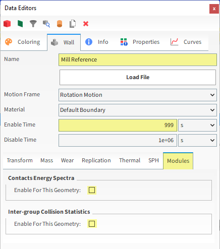
Since the original geometry will be modified by the wear model, we will create a reference geometry for comparison purposes.
From the Data panel, right-click Mill and then select Duplicate. The duplicate will appear as a new Mill <01> item.
Select this new item and then from the Data Editors panel, change the Name to Mill Reference.
Also, increase the Enable Time value. This way, the geometry will be visible during the simulation but not included in calculations.
Finally, from the Modules sub-tab, clear both the checkboxes.
For the Materials step, we will create two new Materials:
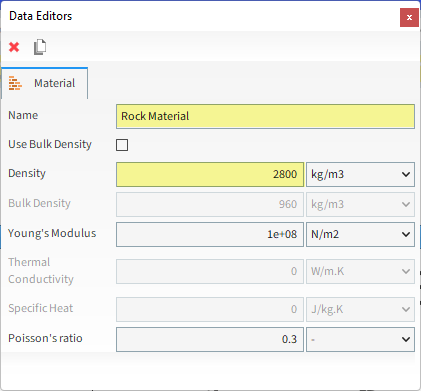
One for the ore (Rock Material)
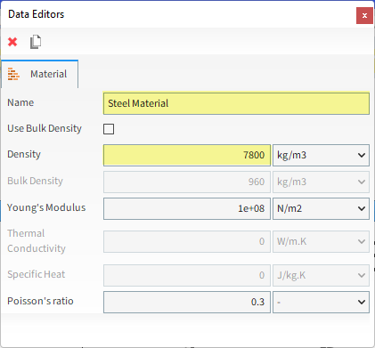
Another for the grinding media (Steel Material)
The Default Boundary Material will be used for the mill slice geometry.
Note: The values for this Material will be left as default.
The other two default Materials (Default Particles and Default Belt) will not be used in this tutorial.
To create the new Materials, complete the following instructions:
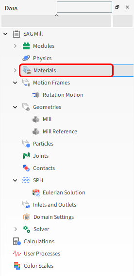
From the Data panel, right-click Materials, and then select Create Solid Material.
Repeat this step once more so that you have two new entries. Material <04> and Material <05> are created under Materials.
Select one of the new Materials and then from the Data Editors panel, change the Name and Density values. Repeat this step for the second new Material.
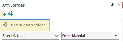
Now let's set the interaction properties for the materials:
Select Materials Interactions in the Data panel.
Adjust the parameters for each combination, according to the values shown below.
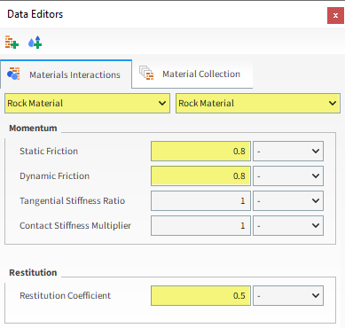
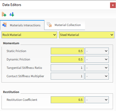
Let the values as default for the other combinations.
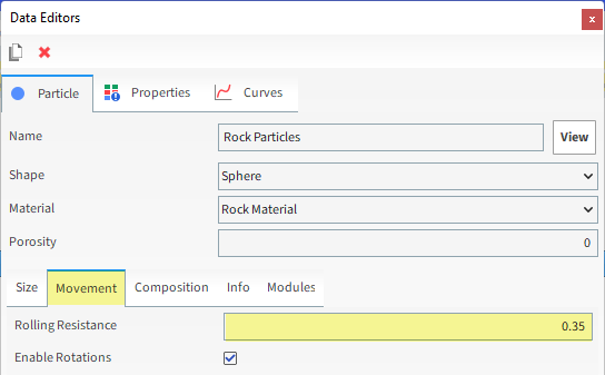
For the Particles step, we will create two new sphere-shaped particle groups with some added rolling resistance. These will represent the ore and grinding media.
To create the Rock particle group, do the following:
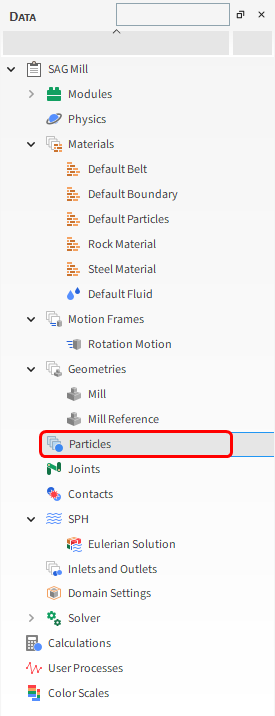
From the Data panel, right-click Particles and then select Create Particle. A new particle group is created under Particles.
Select the newly created Particle <01> entry and then from the Data Editors panel, on the main Particle tab, modify the Name and Material.
From the Size sub-tab, click the green plus button (Add) until you have three size distribution rows. For each row, define the Size (in m) and Cumulative %.
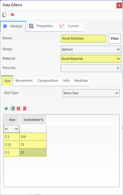
From the Movement sub-tab, define Rolling Resistance.
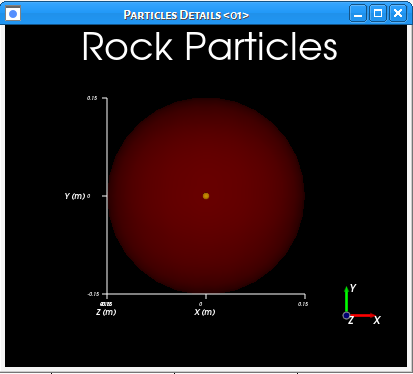
To visualize the newly created particle, the click the View button. A new Particles Details window will appear showing the particle geometry.
For the Steel Particles, do the following:
Create a second new Particle set by right-clicking Particles and selecting Create Particle.
Select this new Particle set, and then from the Data Editors panel, do the following:
On the main Particle tab, define the Name and Material.
From the Size sub-tab, define Size.
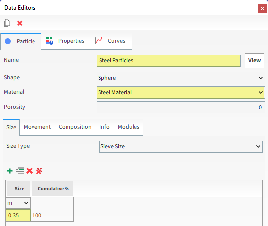
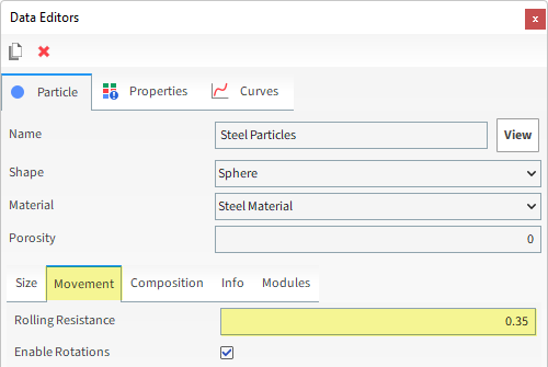
From the Movement sub-tab, define Rolling Resistance.
For the Inlets and Outlets step, we will create a Volumetric Inlet, which enables us to fill a spherical region with closely packed particles into the simulation all at one time.

When compared with the traditional Particle Inlet method, using Volumetric Inlet has the primary benefit of ensuring that the particle bed will already be formed in the mill at the start of the simulation.
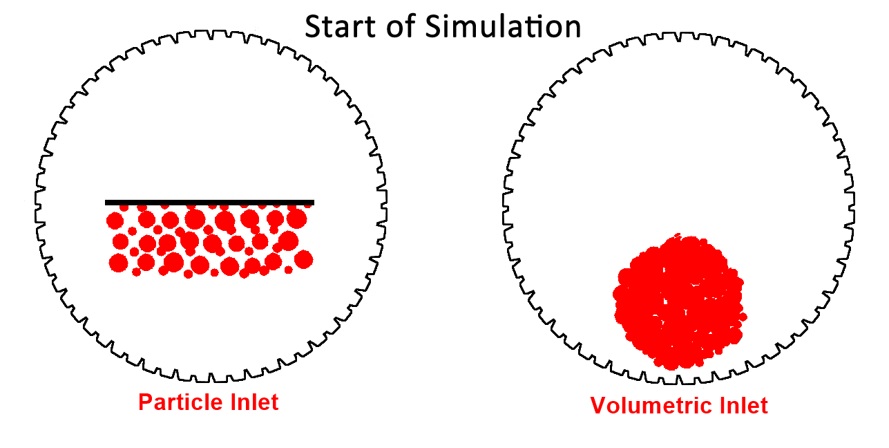
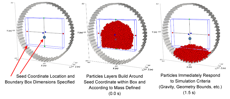
When defining a Volumetric Inlet, it is important to understand the following components:
Seed Coordinate: Location of a point around which layers of particles are built.
Mass: The target mass of particles that you want built around the Seed Coordinate.
Bounds: Defines the physical limits by which the particle layers will be constrained.
The limits must include Box Bounds, which can be defined manually using coordinates, or can be automatically calculated by Rocky using the limits of one or more imported Geometries that you select.
The limits may also include the walls of one or more Geometries within your simulation.
For this tutorial, we'll create a Volumetric Inlet constrained only by the mill geometry.
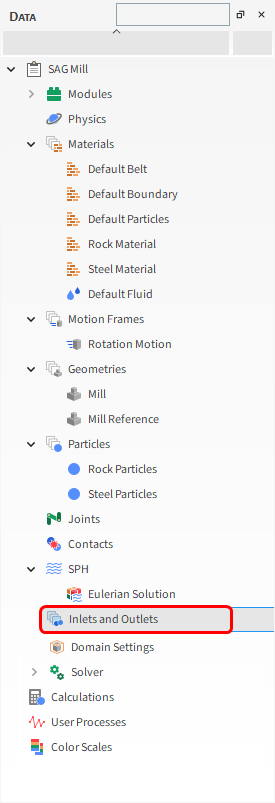
From the Data panel, right-click Inlets and Outlets and then select Create Volumetric Inlet.
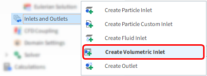
A new entry will be created under Inlets and Outlets.
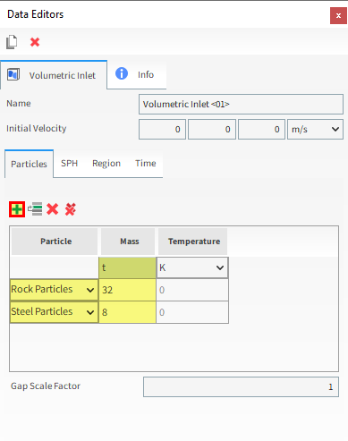
Select the newly created Volumetric Inlet <01> entry, and then from the Data Editors panel, on the Particles sub-tab, click the Add button (green plus) twice to create two entry rows.
For each row, select the Particle group name from the drop down list and then define the Mass in t.
From the Region sub-tab, do the following:
Define the Seed Coordinates.
From the Geometries list, enable the Mill checkbox.
Enable the Use Geometries to Compute checkbox.
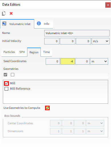
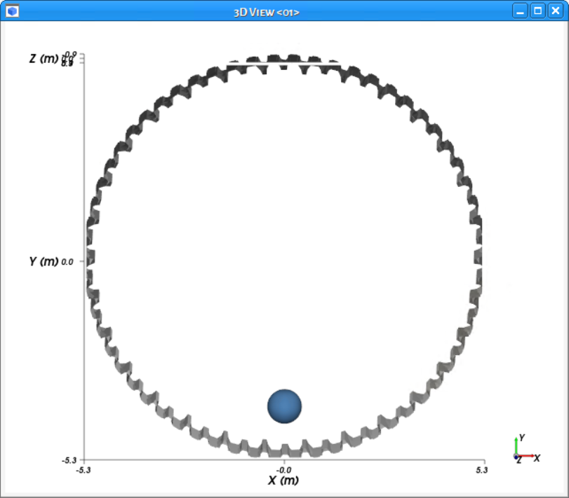
Tip: You can visualize the Seed Point (blue dot) and geometry bounds (white box) in a 3D View window.
A Contact in Rocky refers to a specific location on a geometry or particle that has experienced a collision with another particle during the simulation.
Always during processing, Rocky calculates and makes use of Contacts data. But to save file space, you can choose whether or not to keep it.
For this tutorial, we will enable the collection of the Contacts data so that we can post-process it later.
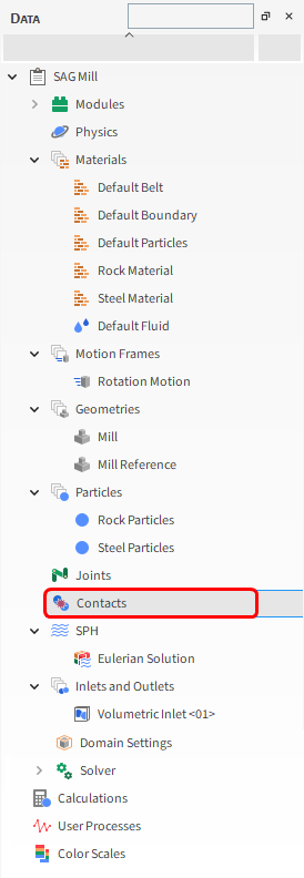
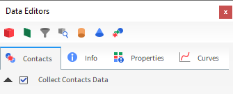
From the Data panel, select Contacts and then from the Data Editors panel, select the Contacts tab.
Enable the Collect Contacts Data checkbox.
For the Domain Settings step, we will define a Cartesian Periodic Domain to recycle particles that leave one side of the mill slice back into the simulation from the opposite side.
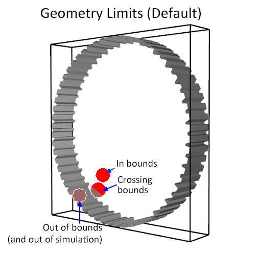
By default, Periodic Domain is turned off and Rocky automatically creates a domain box based upon the Geometries boundary limits.
Any particle that leaves those limits is eliminated from the simulation.
These domain settings would not work for the mill slice as all particles would quickly be eliminated through the open ends of the geometry (as shown).
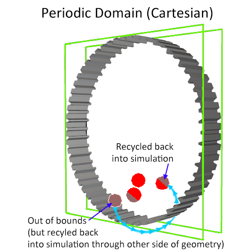
For this case, we need Rocky to put any particles that leave the mill slice back into the mill slice.
To do this, we will define a Cartesian Periodic Domain at the extreme ends of the mill slice geometry.
By doing so, any particles that leave one side of the mill slice are introduced back into the simulation from the other side (as shown).
To define this domain, do to the following:
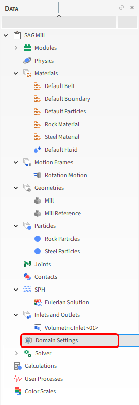
From the Data panel, click Domain Settings.
From the Data Editors panel, set the Periodic Domain Type and the Periodic Direction.
Also, ensure the Periodic at Geometry Limits checkbox is enabled.
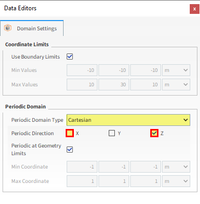
Tip: In order for a periodic Cartesian domain to be representative, the distance between the Min Coordinate and Max Coordinate values must be at least 2.5 times the width of the largest particle size.
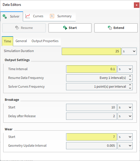
From the Solver | Time tab, do the following:
Define the Simulation Duration.
Under Output Frequencies, define Simulation (as shown).
Under Wear, set the Start time (as shown).
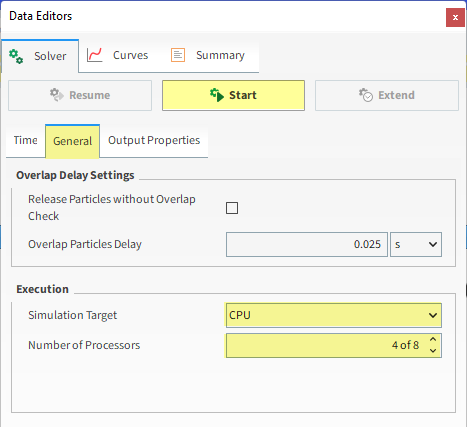
From the General sub-tab, under Execution, do the following:
Select CPU (or GPU/Multi GPU) as Simulation Target.
Set the Number of Processors (or Target GPU(s)).
Note: For this tutorial, CPU will be faster due to the low particle count.
Click the Start button.
Once you click Start, the Simulation Summary window will be displayed.
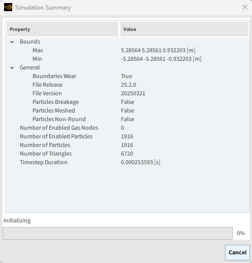
Once initialization is complete, this screen will close automatically and Rocky will process your simulation.
Tip: You can find this information later on the Solver | Summary tab on the Data Editors panel.
Click the Refresh button (or use the Auto Refresh checkbox) to see the results in a 3D View window during processing.
Particle states can be viewed in real time as the simulation progresses.
The speed of the simulation depends on various factors such as:
Number of mesh elements used to define the geometry
Number of contacts in the simulation domain at any time
Smallest particle size and material stiffness
The particle shape and the number of vertices used to define the shape
Frequency of file output
This completes Part A of this tutorial.
For further information on any topic presented, we suggest searching the User Manual, which provides in-depth descriptions of the tools and parameters.
To access this manual, from the main Toolbar click Help, point to Manuals, and then click User Manual.
Rocky was used to set up and process a SAG Mill slice simulation that models wear and collects energy spectra data.
During this tutorial, it was possible to:
Use Modules to collect collision statistics, particle energies, and energy spectra data.
Use Motion Frames to set up a rotation motion.
Define basic surface Wear modification parameters.
Define a Volumetric Inlet.
Set Contacts data to be collected during processing.
Set up a Cartesian Periodic Domain for a mill slice geometry.
What's Next? If you completed this tutorial successfully, then you are ready to move on to Part B and post-process this project.
The main purposes of this tutorial are to use the results from the mill slice simulation we created in Part A to learn how to:
Visualize the wear modification to the surface of the geometry.
Visualize particle trajectories and properties derived from contacts.
Note: We will analyze the particle energies and particle energy spectra data later in Part C.
You will learn how to:
View Wear modification results
Export a worn geometry profile to an .stl file
Display particle trajectories
Visualize Contacts data
Define Eulerian Statistics
And you will use these features:
Rendered Geometry Export
Custom Properties
User Processes, including:
Plane
Particles Trajectories
Eulerian Statistics
Cylinder
This tutorial assumes that you are already familiar with the Rocky user interface (UI) and with the project workflow.
If this is not the case, please refer to Tutorial 01 – Transfer Chute for a basic introduction about Rocky usage before beginning this tutorial.
If you are not sure which Rocky license you have, contact your IT Administrator or Rocky Support for assistance.
If you completed Part A of this tutorial, ensure that Rocky project is open. (Part B will continue from where Part A left off.)
If you did not complete Part A, do all of the following:
Download the
dem_tut04_files.zipfile here .Unzip
dem_tut04_files.zipto your working directory.Open Rocky 2025 R2. (Look for Rocky 2025 R2 in the Program Menu or use the desktop shortcut.)
Important: To make use of the Rocky project file provided, you must have Rocky 2025 R2 or later. If you have an earlier version of Rocky, please upgrade Rocky to the latest version, or complete Part A from scratch.
From the Rocky program, click the Open Project button, find the dem_tut04_files folder, then from the tutorial_04_A_pre-processing folder, open the tutorial_04_A_pre-processing.rocky file.
Process the simulation. (From the Simulation toolbar, click the Start button.)
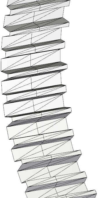
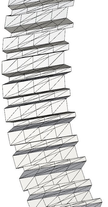
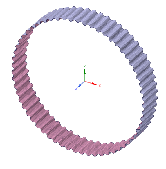
After processing is complete, the geometry surface will appear to be worn away due to shear contact with the particles.
Comparing the profiles of the worn geometry with the reference geometry you duplicated in Part A (as shown) can help you better identify what changed.
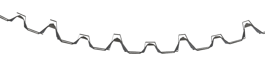
Tip:
To see the reference, rotate the view slightly with your mouse. (In this case, the orthogonal view in the Z-direction is parallel to the reference surface so the reference won't be visible by default.)
To hide the particles from the 3D View window, click the eye icon to the right of Particles in the Data panel.

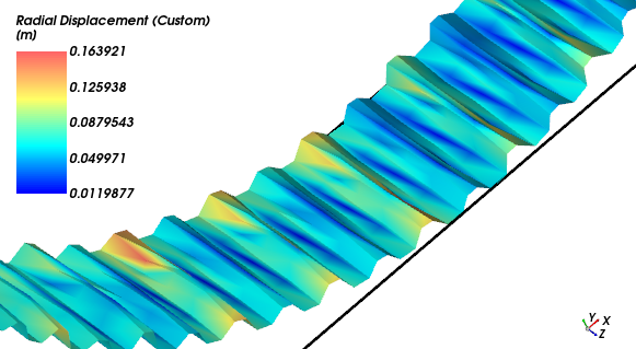
Besides comparing the profiles, another way to analyze the effects of wear is by quantifying the radial displacement of the geometry nodes.
For example, to identify the regions in which the surface wear was most severe, do the following:
From the Data panel, select the Mill geometry.
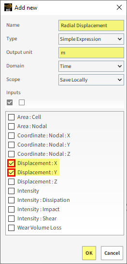
From the Data Editors panel, select the Properties tab and then from the upper right corner, click the Add new custom property button.
From the Add new dialog, define the Name and Output unit; from the Inputs box, enable the checkboxes for Displacement : X and Displacement : Y; and then click OK.
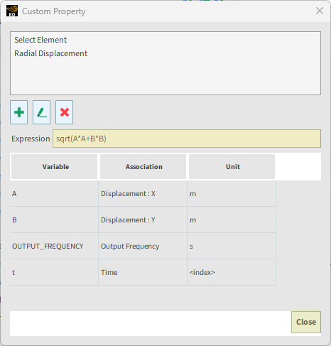
From the Custom Property dialog, enter the Expression (as shown), and then click Close.
From the Properties tab for the Mill geometry, drag-and-drop the newly created Radial Displacement (Custom) property onto the 3D View.
Tip: Use the Data panel eye icon to hide the Mill Reference geometry from the view.
You can also analyze the Radial Displacement on a cut plane of the liner profile.
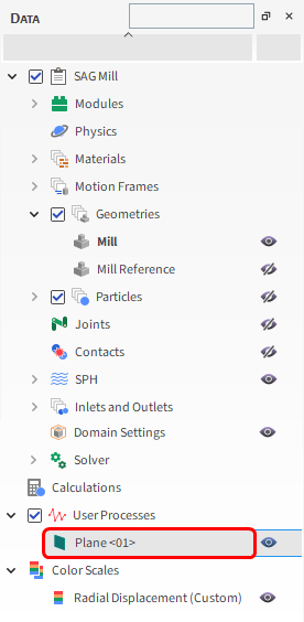
From the Data panel, under Geometries, right-click Mill, point to Processes, and then click Plane.
From the Data panel, under User Processes, select the new Plane <01> entry.
From the Data Editors panel, on the main Plane tab, define the Plane Origin and Orientation | Angle and Vector (as shown).
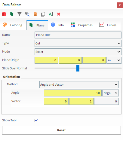
From the Coloring tab, expand the Edges section, and then define the Property and Width values (as shown).
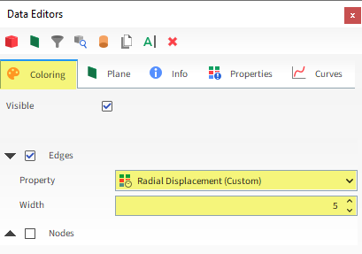
You can view the results in a 3D View window (as shown).
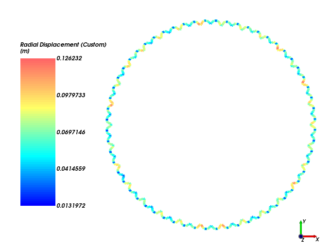
Tip: You may need to use the Data panel eye icon to hide the Mill and Mill Reference geometries from the view.
One final way you can analyze your worn geometry is by exporting it out of Rocky and viewing it in CAD or other 3D graphics program.
From the Time toolbar, select the output for which you want to export worn geometries (as shown).

From the Data panel, under Geometries, right-click Mill, point to Export, and then click Rendered Geometry (as shown).
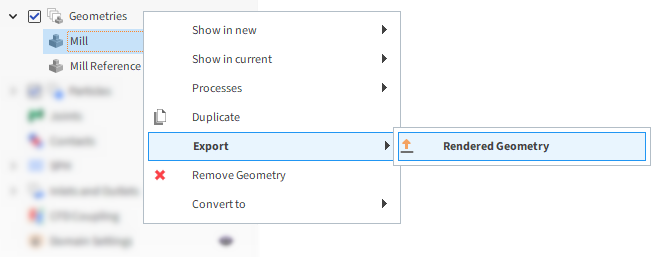
From the Select output unit dialog, define the Output Unit (as shown), and then click OK.
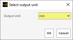
From the Select target STL file dialog, enter a File name and choose a location to save your file, and then click Save.
You can now open your saved .stl file in a CAD program, such as Ansys Discovery.
To analyze the path of the particles, follow these steps:
From the Data panel, right-click Particles, point to Processes, and then select Particles Trajectory.
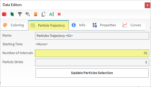
From the Data Editors panel, select the Particle Trajectory tab.
Define the Number of Intervals.
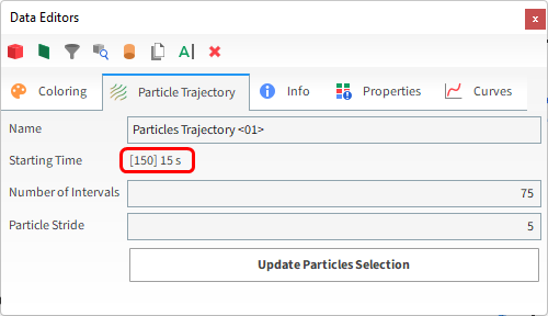
Set the value for the Starting Timestep by doing the following:
From the Time toolbar, select the Output from which you want to begin particle trajectories (as shown).

From the Particle Trajectory tab, click the Update Particles Selection button.
The Timestep you choose now appears in the Starting Timestep field (as shown).
Number of Timesteps: Defines how many future timesteps for which you want to track the particles. The higher the value, the longer the trajectory will be.
Keep in mind that the Starting Timestep value you selected from the Time toolbar should be at least the Number of Timesteps before the end of the simulation.
Particle Stride: Defines how the particles will be sampled. One out of n particles will be tracked, where n is the size of the sample. The higher the value, the lower will be the number of trajectories. If 1 is set, all the particles will be tracked.
Now to visualize the trajectories, we'll show them in a 3D View:
From the Data panel under User Processes, right-click Particles Trajectory <01>, point to Show in new, and then click 3D View.
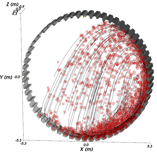
The default view that appears is not ideal for viewing trajectories for the following reasons:
It shows Particles, which get in the way of seeing the trajectory vectors.
It shows the trajectories in black on a black background.
Fix these issues with the view by doing the following:
To hide the Particles, from the Data panel, click the eye icon next to Particles.
Note that even if you hid Particles on your first 3D View, you will have to repeat this process for each new 3D View.
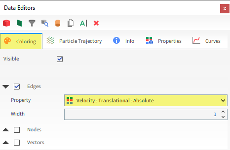
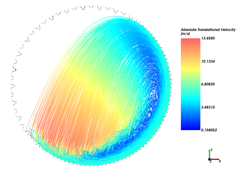
To color the trajectories by particle velocity, from the Data Editors panel, select the Coloring tab, and then under Edges, select the Property type of Absolute Translational Velocity (as shown).
To change the background color, right-click on the 3D View, point to Background color, and then click White.
To change the font color, right-click on the 3D View, point to Font color, and then click Black.
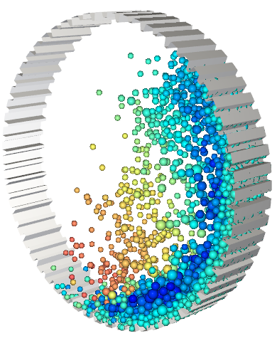
By using the Eulerian Statistics User Process, discrete Properties can be converted into continuous values by averaging the values over discretized regions.
Eulerian Statistics can only be created for a Cube or a Cylinder User Process.
For this tutorial, a Cylinder will be created for this analysis.
From the Data panel, right-click Particles, point to Processes, and then select Cylinder.
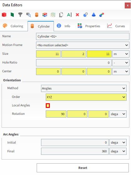
The Cylinder (and Cube) User Processes can be manually changed using the 3D view, or adjusted using their parameters. For this case, we'll enter exact values.
From the Data Editors panel, select the Cylinder tab and then enter the Size, Center, Orientation | Method, Local Angles, and Rotation values (as shown).
From the Data panel under User Processes, right-click the new Cylinder <01> entry, point to Processes, and then select Eulerian Statistics.
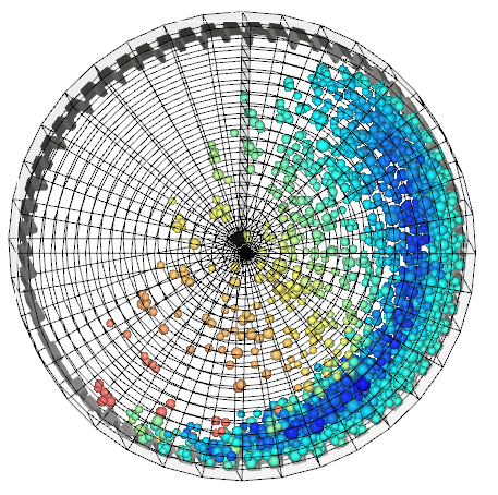
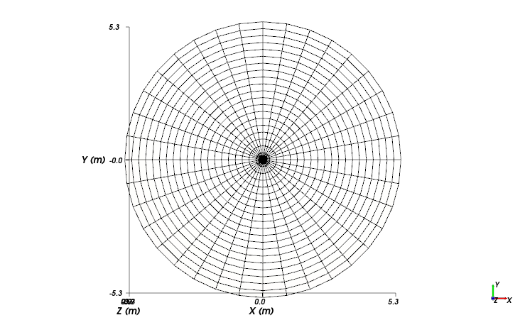
From the Data Editors panel, on the Eulerian Statistics tab, enter the Radial, Tangential and Axial Divisions.
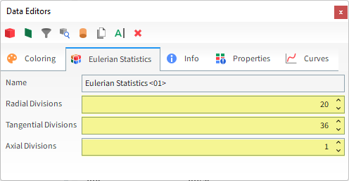
This will discretize the Cylinder into 36 circular sectors, each one divided in 20 bins in the radial direction. A single bin is defined in the axial direction, as shown on the following slide.
Note: You may have to use the Data panel eye icons to hide other data (such as Particles or Particles Trajectories) that you no longer wish to see.
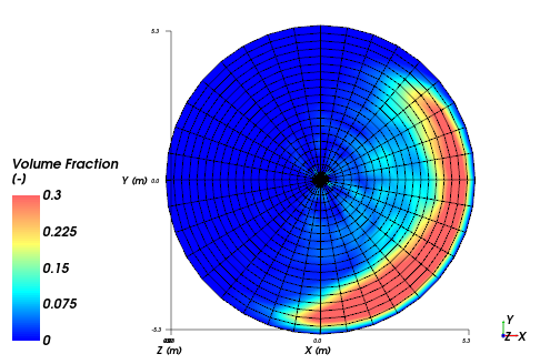
Once the Eulerian Statistics is created, you can modify which Properties are shown through the Colorings tab.
For example, under Faces select the Property called Volume Fraction.
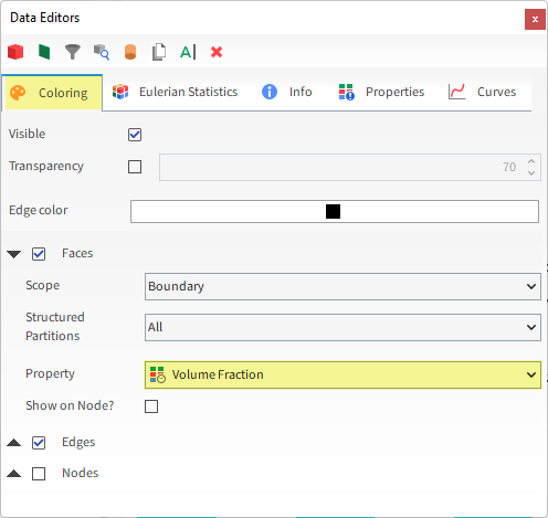
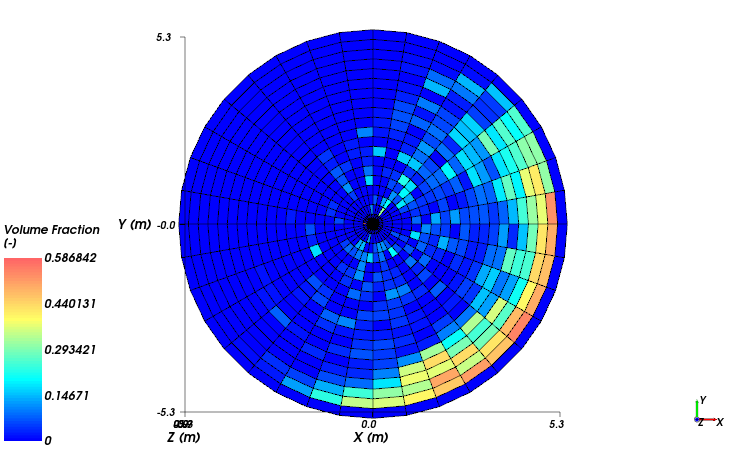
Note: The values you end up with are time dependent, and the ones you get in your project may vary slightly from the ones shown in this Tutorial.
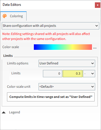
To better visualize the data, you can adjust the limits of the color scale.
From the 3D View window, right-click the color scale, point to Limits options, and then select User Defined.
From the Coloring tab on the Data Editors panel, set the Limits values.
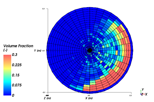
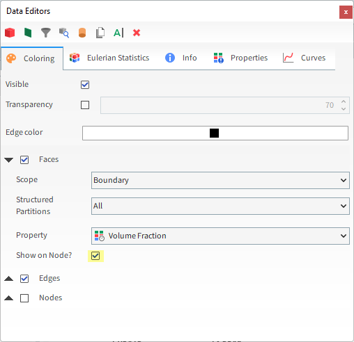
To see a continuous display of the plotted Properties, you can also enable Shown on Node? option.
From the Data panel, under User Processes, select Eulerian Statistics <01> and then from the Data Editors panel, select the Coloring tab.
Under Faces, enable the Show on Node? checkbox (as shown).
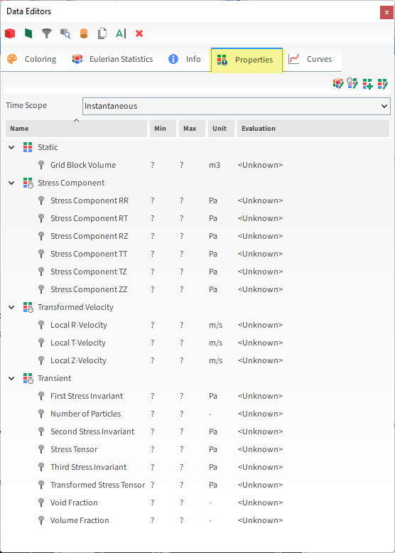
On the Properties tab for Eulerian Statistics, several new properties are available to plot on the Eulerian bins, including:
Static properties
Transformed Velocity properties
Transient properties
Stress Component properties
Important: Important: To be able to analyze Stress Components, you must have enabled the Collect Contacts Data checkbox from Contacts entity on Data panel prior to processing your simulation.
As a reminder, we took this step in Part A, so this data should be now available to analyze.
This completes Part B of this tutorial.
For further information on any topic presented, we suggest searching the User Manual, which provides in-depth descriptions of the tools and parameters.
To access this manual, from the main Toolbar click Help, point to Manuals, and then click User Manual.
Rocky was used to post-process a simulation of a rotating SAG Mill slice.
During this tutorial, it was possible to:
Visualize surface Wear modifications, and compare them to the original wall geometry.
Export the worn geometries to an .stl file for further analysis outside of Rocky.
View the Trajectory of the particles within the mill.
Define a Cylinder User Process.
Evaluate the particle volume fraction in various regions of the mill slice by using Eulerian Statistics.
What's Next? If you completed this tutorial successfully, then you are ready to move on to next tutorial.
The purpose of this tutorial is to evaluate the energy balance of the rotating SAG Mill slice simulation we performed earlier in Part A.
You will learn how to analyze the following Curves:
Energy Spectra
Boundary Collision Statistics Power
Inter-group Collision Statistics Power
Particle Instantaneous Energies Energy
And you will use these features:
Cross Plots
Custom Curves
Output Variables
This tutorial assumes that you are already familiar with the Rocky user interface (UI) and with the project workflow.
If this is not the case, please refer to Tutorial 01 Transfer Chute for a basic introduction about Rocky usage before beginning this tutorial.
If you are not sure which Rocky license you have, contact your IT Administrator or Rocky Support for assistance.
If you completed Part A (or Part B) of this tutorial, ensure that Rocky project is open. (Part C will continue from where either Part A or B left off.)
If you did not complete Part A (nor Part B), do all of the following:
Download the
dem_tut04_files.zipfile here .Unzip
dem_tut04_files.zipto your working directory.Open Rocky 2025 R2. (Look for Rocky 2025 R2 in the Program Menu or use the desktop shortcut.)
Important: To make use of the Rocky project file provided, you must have Rocky 2025 R2 or later. If you have an earlier version of Rocky, please upgrade Rocky to the latest version, or complete Part A from scratch.
From the Rocky program, click the Open Project button, find the dem_tut04_files folder, then from the tutorial_04_A_pre-processing folder, open the tutorial_04_A_pre-processing.rocky file.
Process the simulation. (From the Simulation toolbar, click the Start button.)
Size reduction is a very energy-intensive process, representing a major percentage of mineral beneficiation costs.
Although mills have great energy consumption, only a small part of this energy is converted into actual particle fragmentation.
Because of this, it is crucial to understand how power is consumed during comminution processes in order to improve grinding efficiency and reduce costs.
One way this can be accomplished in Rocky is by using a tool called Energy Spectra.
Unlike breakage simulations, which require additional computational costs to calculate and visualize each individual broken fragment, Energy Spectra uses energy statistics of particle collisions to predict breakage and attrition rates in a graphical format.
This provides answers to breakage questions faster by avoiding the computationally intensive visualization step of the particles actually breaking.
In Energy Spectra plots, the collision data collected during a simulation is classified based on the energy levels of the individual collisions and then displayed accordingly.
Three types of collision energy can be evaluated using Energy Spectra plots:
Dissipated energy: The fraction of the mechanical energy of the particle transformed irreversibly into other forms of energy during a collision.
Impact energy: The maximum collision energy transferred during the normal loading phase. This kind of energy is considered in the instantaneous breakage models to evaluate breakage.
Shear energy: The work done by the tangential contact forces during a collision. This kind of energy is used in the abrasive wear models.
Depending upon the source of the energy values considered, two types of Energy Spectra plots are available in Rocky:
Contacts energy spectra: Energy values are collected collision-wise and are classified by contact pair (particle and/or geometry).
Particles energy spectra: Specific energy values are collected particle-wise, and are classified by size and particle group.
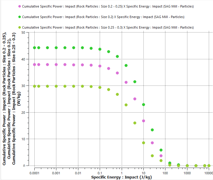
To demonstrate how to evaluate breakage rate using an Energy Spectra curve, consider Cumulative Specific Power : Impact as it relates to the energy used in the instantaneous breakage models:
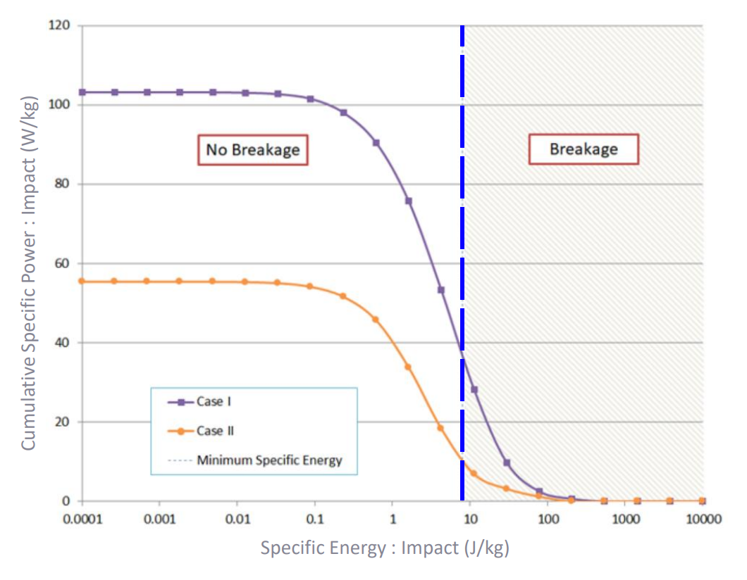
The blue dashed line defines the minimum specific energy for a certain particle to break.
All collisions with specific impact energy higher than this value may lead to breakage. The remaining collisions do not lead to breakage.
The power consumed that actually promotes particle fragmentation is given by the corresponding Y-value.
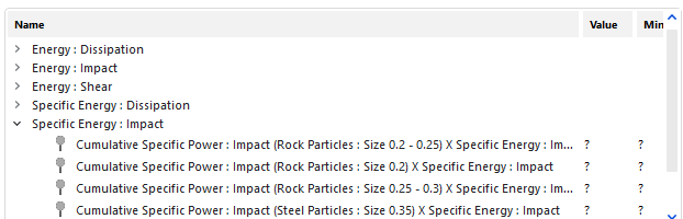
After the simulation is complete, information about Energy Spectra will be available on the Curves tab for the Particles entity.
From the Data panel, select Particles and then from the Data Editors panel, click the Curves tab.
The new Energy Spectra Curves will be displayed under two separate groups:
Energy, which shows the Contacts energy spectra energy curves.
Specific Energy, which shows the Particle energy spectra curves.
Both Energy and Specific Energy are separated into Impact, Shear, and Dissipation energies.
For Energy (Contacts energy spectra), each pair composed of either Particles & Particles or Particles & Geometries will present a separate Energy Spectra.
Energy Curves are displayed in three ways:
Cumulative Power: Displays the sum of all power coming from a collision with energy greater than a specified energy.
Power: Displays the time average of energy resulting from all collisions of that type and pair.
Rate: Displays the mean frequency of collision for that type and pair.
Cumulative sums and averages making use of Cumulative Power, Power, and Rate are computed from the Energy Spectra Start time (which is defined on the Solver | Energy Spectra tab) to the current timestep.
For Specific Energy (Particle energy spectra), each Particle set and Particle Size group will present a separate Energy Spectra.
Specific Energy curves are displayed only as Cumulative Specific Power, which displays the sum of all specific power coming from a collision with energy greater than a specified energy level.
Cumulative Power is computed from the Energy Spectra Start time (which is defined on the Solver | Energy Spectra tab) to the current timestep.
To plot the curves, follow these steps:
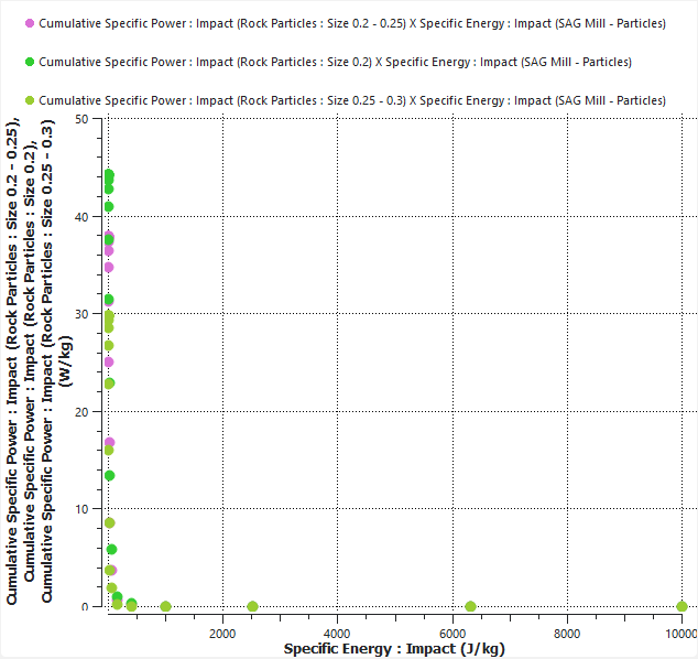
Under Specific Energy : Impact right-click the first Cumulative Specific Power : Impact entry and then click Show curve in new Plot. (Or click Show curve in selected Plot if a plot is already created.)
A new Cross Plot window appears with the data.
Plot the next two Cumulative Specific Power: Impact entries on the same plot so that it contains all 3 Rock Particles size ranges.
Change the axis display option by right-clicking the grid and then under Axes Layout, choosing By Quantity.
To edit the scale, do the following:
Right-click in the plot area and then select Settings.
From the Window Editors panel, select the Axes tab and then from the Axis box, select Specific Energy : Impact (J/kg).
Under Values, ensure Limits are set to Automatic.
Under Scale Options, enable the Logarithmic Scale checkbox.
Select the last output from the Time Toolbar.
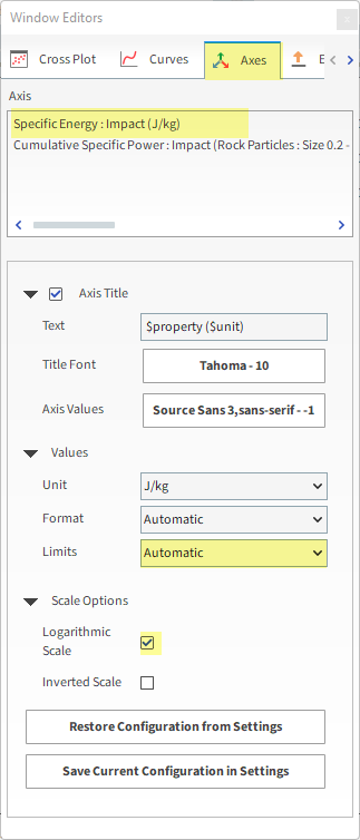
The resulting plot is shown on the next slide.
Repeat this same procedure to show Energy : Impact values:
In the Data Editors, on the Curves tab under Energy : Impact, you can repeat the same procedures to create a new Cross Plot showing both the Power: Impact and Cumulative Power : Impact of the collisions between Rock Particles and Mill (only). (Resulting plot shown.)
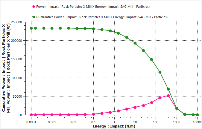
Note: The Logarithmic Scale is enabled only for the horizontal axis in the plots shown in these analyses.
Tip: Add lines to your points by right-clicking a point on the plot and then choosing the Edit option. From the Edit Curves dialog that appears, choose the line options you want under Pen Style. Here, Solid Line is selected for both Curves.
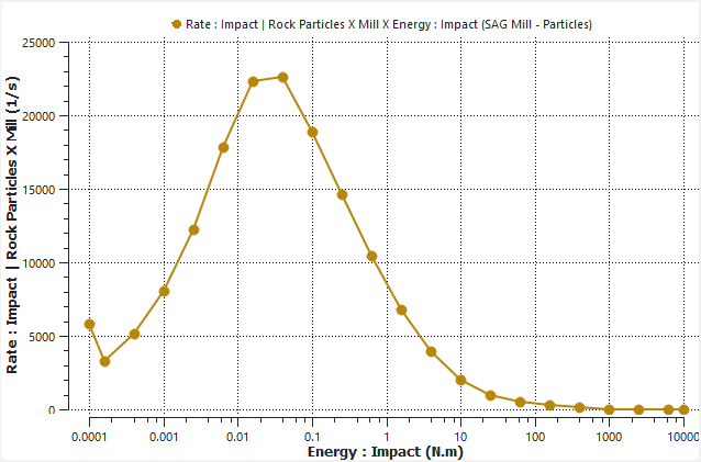
Also under Energy : Impact, create a new Cross Plot of the Rate : Impact between Rock Particles and Mill (only). (Resulting plot shown.)
In Rocky, it is possible to analyze how the energy is distributed in the system.
In this tutorial, the energy supplied by the mill is transferred to the particles. Part of this energy is dissipated and another part is transformed into mechanical energy. The equation below shows the Energy Balance of this system:
 | (4–1) |
In terms of Power:
 | (4–2) |
Where:
 is the energy supplied by the mill.
  is the dissipated energy.
  is the variation in mechanical energy of the particles.
  is the dissipated power.
  is the power supplied by the mill.
  is the time interval in which the power was applied.
In Rocky, the power supplied by the mill and the mechanical energy variation of the particles are directly obtained.
The dissipated energy can be obtained directly or by using power curves depending upon how we want to analyze it.
In this way, we have two equations that can be used to calculate the Energy Balance:
 | (4–3) |
 | (4–4) |
For this tutorial, we will use Output Variables to compute the terms of these equations.
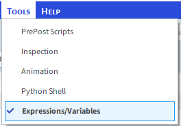
From the Tools menu, ensure that Expressions/Variables is enabled.
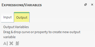
From the Expressions/Variables panel, select the Output tab (as shown).
The value can be obtained from the Mill
geometry by using the Power Curve.
Note: This Curve is available only if the Intensities checkbox is enabled on the Boundary Collision Statistics module prior to processing, which we did in Part A.
From the Data panel, select Mill and, from the Data Editors panel, select the Curves tab.
Drag-and-drop the Power Curve onto the Output tab of the Expressions/Variables panel.
From the Output tab, select the newly added Power entry, and then click the Edit
 button (as
shown).
button (as
shown). 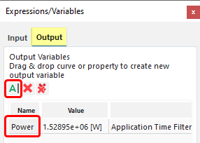
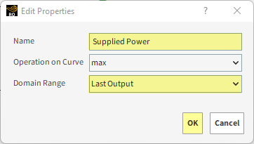
From the Edit Properties dialog, enter the Name and Domain Range (as shown), and then click OK.
The power supplied by the mill during the last timestep is shown in the Output tab.
The value can be obtained from any of the following Particles data:
Energy Delta Curve
Energy : Kinetic : Rotational Property
Energy : Kinetic : Translational Property
Energy : Potential Property
Note: These Curves and Properties are available only if the Particles Instantaneous Energies module is enabled prior to processing, a step which we took in Part A of this tutorial.
For this tutorial, we will use the Energy Delta to compute the Mechanical Energy variation contribution to the energy balance.
The Energy Delta is the variation of the Mechanical Energy in a given timestep.
Since the term that involves the variation of Mechanical
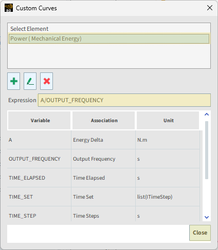
Energy is divided by , we can create a Custom Curve of
Energy Delta divided by the Output
Frequency (which is ).
To calculate the mechanical energy balance, follow these steps:
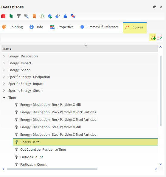
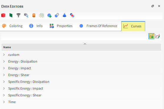
From the Data panel, select Particles, and then from the Data Editors panel, select the Curves tab.
Under Time, select the Energy Delta Curve, and then click the Add new custom curve button (as shown).
From the Add new dialog, define the Name and Output Unit, and then click OK (as shown).
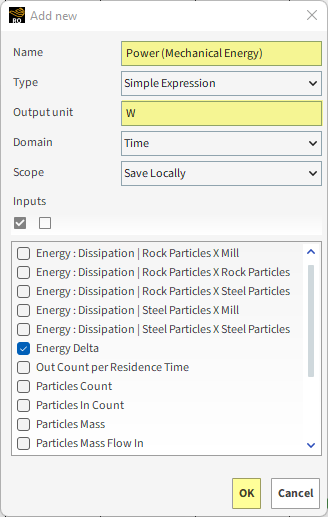
From the Custom Curves dialog, enter the Expression, and then click Close (as shown).
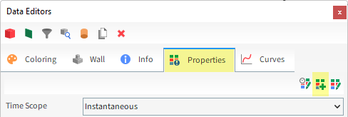
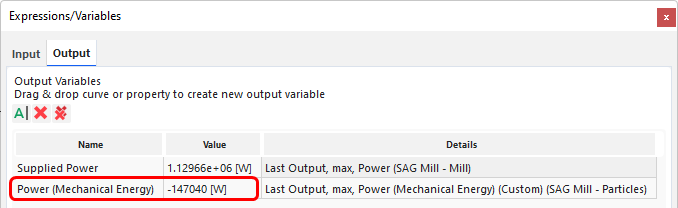
From the Data Editors panel, under custom, drag-and-drop the newly created Power (Mechanical Energy) (Custom) Curve onto the Output tab of the Expressions/Variables panel.
From the Output tab, select the newly added Power_Mechanical_Energy_Custom_ entry, and then click the Edit
button. From the Edit Properties dialog, enter the Name and Domain Range (as shown), and then click OK.
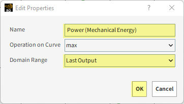
The power transferred to Mechanical Energy during the last output is shown in the Output tab.
Alternate Method:
You can also calculate the Mechanical Energy by summing up the Energy : Kinetic : Rotational and Energy : Kinetic : Translational and Energy : Potential properties from Particles in a Custom Property.
With the Mechanical Energy calculated, compute its variation from 24.9s to 25.0s and then divide it by the time variation.
This should result the same value we've obtained in the previous step.
can be obtained from the following Particles Properties or Curves:
Power : Dissipation
Note: This Property is available only if the Power checkbox is enabled on the Inter-particle Collision Statistics module prior to processing, a step which we took in Part A of this tutorial.
Energy : Dissipation (between pairs of groups)
Note: This Curve is available only if the Energy Dissipation checkbox is enabled on the Intergroup Collision Statistics module prior to processing, a step which we took in Part A of this tutorial.
Cumulative Power : Dissipation
Cumulative Specific Power : Dissipation
Power : Dissipation (listed under Energy : Dissipation)
Note: These Curves are available only if Energy Spectra is enabled prior to processing, a step which we took in Part A of this tutorial.
For this tutorial, we will estimate in two different ways:
By Energy : Dissipation (between pairs of groups)
By Cumulative Power : Dissipation from energy spectra
First, to calculate using Energy : Dissipation (between pairs
of groups), do the following:
From the Data panel, select Particles, and from the Data Editors panel, select the Curves tab and click the Add new custom curve button.
From the Add new dialog, define the Name and the Output Unit, and then under Inputs, enable all the Energy : Dissipation Curves between pairs (as shown), and then click OK.
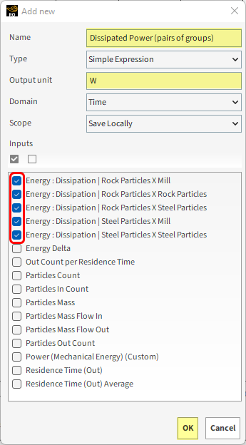
Tip: This should involve 5 separate pairs.
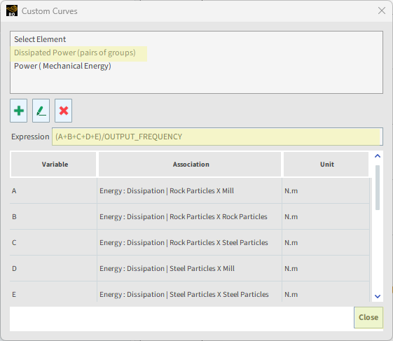
From the Custom Curves dialog, set the Expression, and then click OK (as shown).
From the Data Editors panel, under custom, drag-and-drop the newly created Dissipated Power (pairs of groups) (Custom) onto the Output tab of the Expressions/Variables panel.
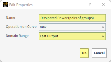
From the Output tab, select the newly added Dissipated_Power_pairs_of_groups_Custom entry, and then click the Edit
button. From the Edit Properties dialog, enter the Name and Domain Range (as shown), and then click OK.
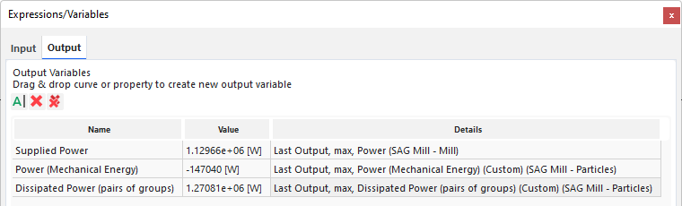
The Dissipated Power during the last timestep is shown on the Output tab.
Now, we recall the Energy Balance equation we stated before:
| (4–5) |
If we compare the values in a spreadsheet, we see that the Energy Balance is satisfied with a difference of ≈ 0.5%.
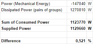
Tip: To analyze the data outside of Rocky, you can copy the values directly out of the Value column and paste them into a spreadsheet program.
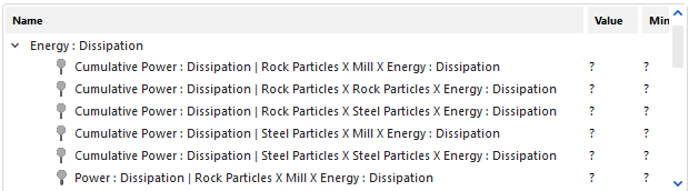
Next we will calculate using the Cumulative Power : Dissipation
from Energy Spectra.
As implied earlier, the Energy Spectra curves are temporal averages.
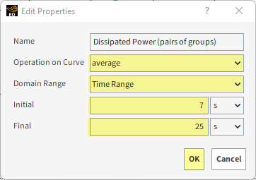
To compare the dissipated power of the two different methods, instead of using Specific Time as the Operation on Curve in the Dissipated Power (pairs of groups) Output variable, we will be using Average from 7 s (Energy Spectra Start) to 25 s (Simulation Duration).
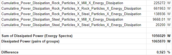
Since the Cumulative Power : Dissipation are cumulative curves, we just have to sum the maximum value of each pair of groups to obtain the Dissipated Power.
Follow the steps below to compare the dissipated power obtained by the Energy Spectra and the Inter-group Collision Statistics calculation methods.
From the Expressions/Variables panel, in the Output tab, double-click Dissipated Power (pairs of groups).
From the Edit Properties dialog box, set Operation on Curve and Domain Range (as shown).
For the Particles entity, from the Data Editors panel, select the Curves tab.
Under Energy : Dissipation, multi-select all the Cumulative Power : Dissipation Curves.
Drag and drop all five Curves onto the Output tab of the Expressions/Variables panel (resulting panel shown).
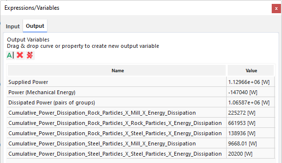
Note: It is not necessary to alter these output variables properties, since the default values already select the maximum value of each curve in the last output.
If we compare the values in a spreadsheet, we see that the difference between the two Dissipated Power calculations is ≈ 1%.
Tips for further exploration:
To compute the Dissipated Power using the Power : Dissipation property from Particles, sum the power dissipated for each particle for each timestep and then average the values from 7s until the end of the simulation.
To compute the Dissipated Power using the Cumulative Specific Power : Dissipation Curves, use the method we used earlier for Cumulative Power : Dissipation but instead, multiply each Curve by the total particle mass for that size range.
To compute the Power : Dissipation Curves, use the method we used earlier for Cumulative Power : Dissipation but instead, sum all the points of the Curve instead of picking only the first point.
This completes Part C of this tutorial.
For further information on any topic presented, we suggest searching the User Manual, which provides in-depth descriptions of the tools and parameters.
To access this manual, from the main Toolbar click Help, point to Manuals, and then click User Manual.
Rocky was used to evaluate the energy balance of a rotating SAG Mill slice simulation.
During this tutorial, it was possible to:
Use a Cross Plot to evaluate Energy Spectra for particles and contacts.
Use the Output Variables to estimate average values of Power and Energy from the following sources:
Boundary Collision Statistics Power Curves
Inter-group Collision Statistics Power Curves
Particle Instantaneous Energies Energy Curves
Contacts Energy Spectra Curves
Particles Energy Spectra Curves
What's Next? If you completed this tutorial successfully, then you are ready to move on to next tutorial.