


(Part A) Set up and process a HPGR simulation using the Boundary Collision Statistics Module, the Ab-T10 breakage model, and the surface wear modification model. Also define a Motion Frame with a free body rotation and spring-dashpot moment.
(Part B) Learn how to collect and analyze particle fragments, create a color map for the shear wear, and calculate and compare the power draw in the rollers.
The main purpose of this tutorial is to set up and process a High Pressure Grinding Roll (HPGR) simulation, with the goal of later (in Part B) analyzing both power and wear data on the boundaries.
In the mining industry, HPGRs are commonly used to reduce the size of hard materials, such as rock and ore, for further processing.
You will learn how to:
Turn on the collection of data related to boundary collisions
Add a default Feed Conveyor
Create a Motion Frame with a Free Body Rotation and Spring-Dashpot Moment
Enable the surface wear modification model
Set up and define a particle group for breakage modeling
And you will use these features:
Boundary Collision Statistics Module
Motion Frames
Surface Wear Modification Model
Ab-T10 Breakage Model
Important: This ADVANCED tutorial contains fewer details, screenshots, and procedures than other Rocky tutorials.
An ADVANCED tutorial is designed for users who are more familiar with the Rocky user interface (UI), and already have a good understanding of the common setup and post-processing tasks.
If you do not already have this level of familiarity, it is recommended that you complete at least Tutorials 01 - 05 before beginning this one.
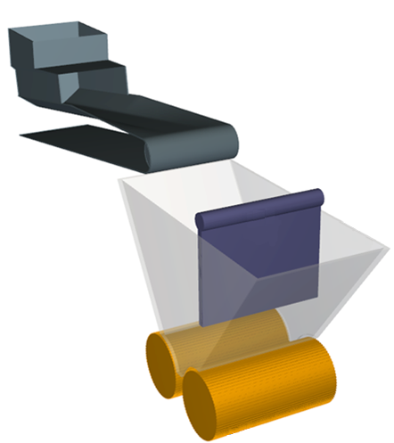
The geometries in this tutorial are composed of:
(1) Feed Conveyor
(2) Hopper
(3) Deflector
(4) Roll 1
(5) Roll 2
For all but the first item, which will come from a conveyor template within Rocky, the .stl files can be found in the tutorial directory.
To begin the steps for this tutorial, do the following:
Download the
dem_tut06_files.zipfile here .Unzip
dem_tut06_files.zipto your working directory.Open Rocky 2025 R2.
Create a new project.
Save the empty project to a location of your choosing.
Use the information in the table that follows to start setting up your Rocky project.
Step Data Entity Editors Location Parameter or Action Settings A Study 01 Study Study Name HPGR B Physics Momentum Numerical Softening Factor 0.1 [-] Tip: If you run into settings or procedures in these tables that you are not yet familiar with, please refer to the Rocky User Manual and/or other Tutorials (via the Introductory Tutorials and Advanced Tutorials) to find the detailed instructions you need.
For the Modules step, we will be turning on the collection of some Boundary Collision Statistics so that we may later analyze Intensities information, such as power and shear.
Tip: Refer to Tutorial 04 – SAG Mill | Part A: Project Setup and Processing for further details on Modules.
Use the information in the table that follows to define your Modules.
Step Data Entity Editors Location Parameter or Action Settings A Modules Modules Boundary Collision Statistics (Enabled) B Modules ﹂Boundary Collision Statistics
Boundary Collision Statistics Intensities (Enabled)
Besides importing the HPGR components, a Feed Conveyor will be added to this tutorial, which will come from a Conveyor Template included by default within Rocky.
Rocky not only allows Custom geometry import but also provides some default geometries that you can add to your projects and then customize.
The Feed Conveyor can input the particles if you associate an inlet to it, so you don't need a separate surface.
From the Data panel, right-click Geometries, point to Conveyor Templates, and then click Create Feed Conveyor.
From the Data Editors panel, define the parameters for the resulting Feed Conveyor <01> item and import the necessary HPGR components by using the information in the table below.
Step Data Entity Editors Location Parameter or Action Settings A Geometries ﹂Feed Conveyor <01>
Geometry Belt Width 1.5 [m] Orientation Belt Incline Angle 10 [dega] Vertical Offset 3 [m] Horizontal Offset -1 [m] Out-of-Plane Offset 1 [m] Feeder Box Front Plane Offset 1 [m] B Geometries Import Wall Deflector.stl, Hopper.stl, Roll 1.stl,Roll2.stl with "mm" for Import Unit
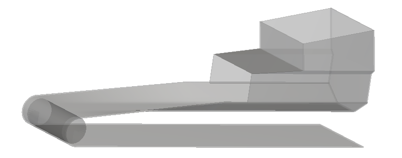
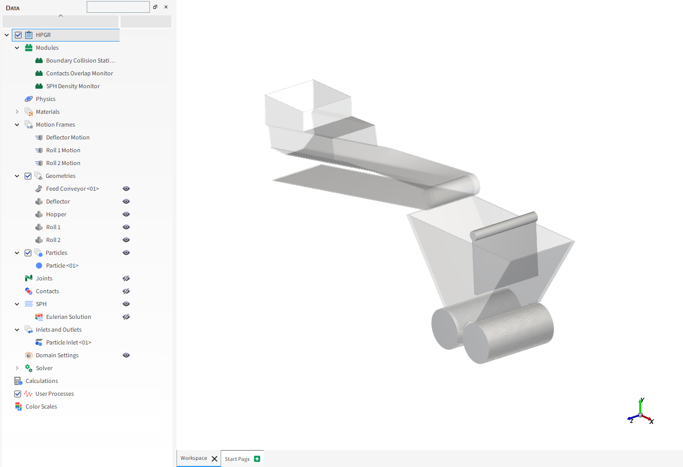
To visualize the geometries, click and drag Geometries from the Data panel, releasing it over the Workspace. The workspace should look similar to the image below.
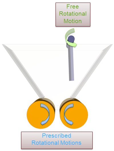
For the Motion Frames step, we will create three separate Motion Frames: one each for the HPGR rolls, and one for the deflector plate.
Both Rolls have rotational movements in opposite directions.
The left roll rotates in a clockwise direction.
The right roll rotates in counter-clockwise direction.
The Deflector has a Free Body Rotation motion around its axis with a Spring-Dashpot Moment resisting the torsional motion.
When the motion Type of Spring-Dashpot Moment (or Spring-Dashpot Force) is selected, you must then prescribe the direction and the coefficients of the Spring/Dashpot.
The moment (M) and force (F) components at the selected direction for this motion will be proportional to the displacement (Spring) and velocity (Dashpot) of the geometry, compared to the original position.
 | (6–1) |
 | (6–2) |
Where:
 and
and  are the Spring Coefficients
  and
and  are the Dashpot Coefficients
  is the Linear Displacement
  is the Linear Velocity
  is the Angular Displacement
  is the Angular Velocity
Use the information in the following table to set up the Roll 1 and 2 Motion Frames for this tutorial:
Step Data Entity Editors Location Parameter or Action Settings A Motion Frames Create Motion Frame B Motion Frames ﹂Frame <01>
Frame Name Roll 1 Motion Add Motion Type Rotation⯆ Initial Angular Velocity 0, 0, -50 [rad/s] C Motion Frames Create Motion Frame D Motion Frames ﹂Frame <01>
Frame Name Roll 2 Motion Relative Position 1.2, 0, 0 [m] Add motion Type Rotation⯆ Initial Angular Velocity 0, 0, 50 [rad/s] Similarly, set up the Deflector Motion Frame.
Step Data Entity Editors Location Parameter or Action Settings E Motion Frames Create Motion Frame F Motion Frames ﹂Frame <01>
Frame Name Deflection Motion Relative Position 1.105, 2.75, 0 [m] Add motion Type Free Body Rotation⯆ Motion Direction Z direction ⯆ Add motion Type Spring-Dashpot Moment⯆ Direction Z direction⯆ Spring Coefficient 1000 [Nm/dega] Dashpot Coefficient 100 [Nms/dega] Once the Motion Frames are created, they can be assigned to their respective geometries.
Step Data Entity Editors Location Parameter or Action Settings G Geometries ﹂Deflector
Wall Motion Frame Deflection Motion⯆ H Geometries
﹂Roll 1
Wall Motion Frame Roll 1 Motion⯆ I Geometries
﹂Roll 2
Wall Motion Frame Roll 2 Motion⯆ To visualize the newly created Frames, click Motion Frames and then click Preview.
Note:
The Feed Conveyor does not need a Motion Frame since its movement is already predefined in the default geometry settings.
Since the Feed Conveyor has motion without displacement and the Free Body Motions can only predict the effects of gravity prior to particle interactions being calculated, you will see only minor movements in the Deflector and more obvious movements on only the two Roll motions.
Since the Deflector has a free body motion, it is important to correctly define the Boundary Mass, Gravity Center and Moment of Inertia properties.
Doing so enables Rocky to properly calculate the resulting accelerations.
In addition, the Surface Wear Modification model will be enabled for the Deflector.
Use the information in the table below to set up the boundary parameters.
Step Data Entity Editors Location Parameter or Action Settings A Geometries ﹂Deflector
Wall | Transform Triangle Size 0.1 [m] … | Mass Boundary Mass 2810 [kg] Gravity Center 1.125, 2.144, 1 [m] Principal Moment of Inercia 1546.4, 8489.87, 705.72 [kg.m2] … | Wear War Model Shear Work Proportionality (Archard's Law) Volume/Shear Work Ration 5e-07 [m3/J]
Next, we will define the interactions between materials.
To set the interaction properties, use the information in the table below.
Step Data Entity Editors Location Parameter or Action Settings A Materials Materials Interactions Default Particles⯆
Default Boundary⯆
Static Friction 0.5 [-] Dynamic Friction 0.5 [-] Materials Interactions Default Particles⯆
Default Particles⯆
Dynamic Friction 0.5 [-]
For the Particles step, we will create a new (rock-like) polyhedron-shaped particle group in a range of sizes, and will define for it Ab-T10 breakage parameters.
Use the information in the table that follows to define these settings.
Step Data Entity Editors Location Parameter or Action Settings A Particles Create Particle B Particles ﹂Particle <01>
Particle Shape Polyhedron⯆ Particle | Size Add row (x2) (1) Size | Cumulative % 0.3 [m] @ 100 [%] (2) Size | Cumulative % 0.2 [m] @ 30 [%] (3) Size | Cumulative % 0.15 [m] @ 10 [%] … | Shape Horizontal Aspect Ratio 1 [-] Number of Corners 15 [-] … | Breakage Enable Breakage (Enabled) Model Ab-T10⯆ Reference Minimum Specific Energy 1 [J/kg] Selection Function Coefficient 0.001 [kg/J … | Breakage | Fragments Minimum Absolute Size 0.05 [m]
Lastly, we will define an inlet and solver information for this project.
Use the information in the table below to continue setting up your project.
Step Data Entity Editors Location Parameter or Action Settings A Inlets and Outlets Create Particle Inlet B Inlets and Outlets ﹂Particle Inlet <01>
Particle Inlet Entry Point Feed Conveyor <01> Particle Inlet | Particles Add row (x1) (1) Particle | Mass Flow Rate Particle <01>⯆ @ 1500 [t/h] C Solver Solver | Time Breakage | Start 3 [s] Breakage | Delay after Release 3 [s] Wear | Start 3 [s] … | General Simulation Target CPU⯆
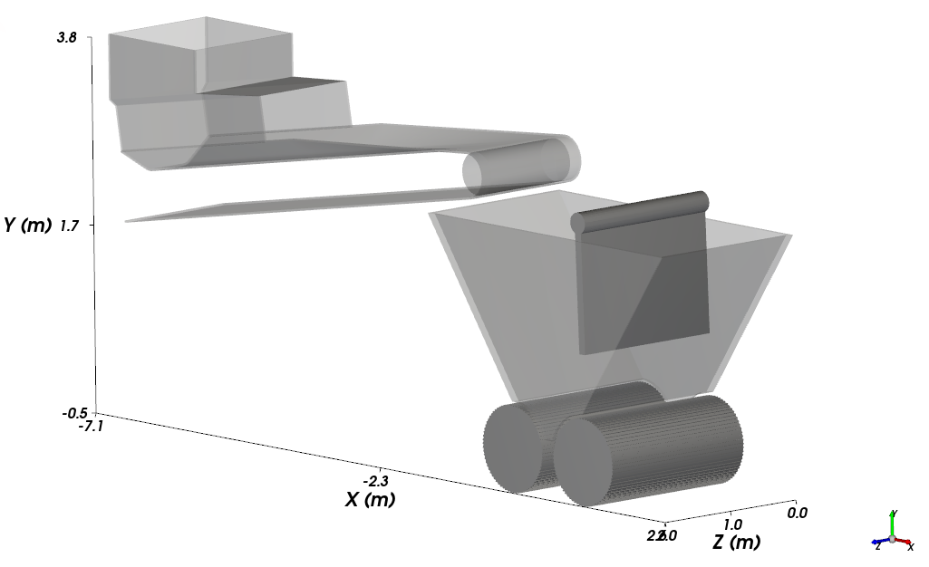
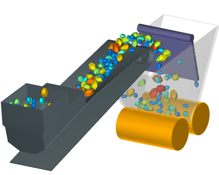
With a 3D View opened, your Data and Workspace should look similar to the image below.
From the Solver entity, click Start.
The Simulation Summary window will be displayed, and then processing begins.
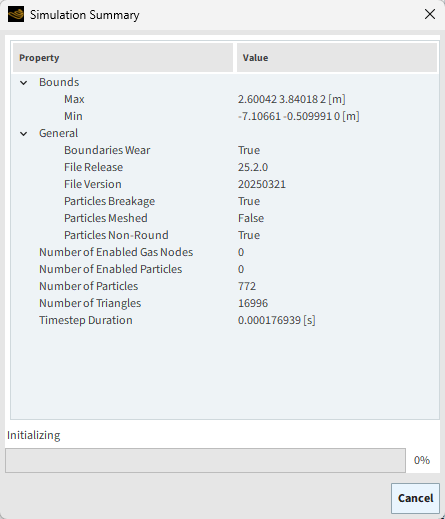
Tip: You can use the Auto Refresh checkbox to view the results during processing.
This completes Part A of this tutorial.
Rocky was used to set up and process an HPGR simulation with the goal of later analyzing both power and wear data on the boundaries.
During this tutorial, it was possible to:
Use Modules to enable the collection of boundary collisions data.
Set up a Motion Frame using a free body rotation and a spring-dashpot moment.
Enable the Surface Wear Modification model.
Enable the Ab-T10 Breakage model.
What's Next?
If you completed this tutorial successfully, then you are ready to move on to Part B and post-process this project.
The main purposes of this tutorial are to analyze the particle fragments, view the surface wear modifications, and compare the power data that we collected in the High Pressure Grinding Roll (HPGR) simulation we processed in Part A.
You will learn how to:
Collect and analyze Particle fragments
Measure and visualize surface displacement
Measure and visualize wear volume loss
Create a color map of Intensity : Shear
Calculate and compare power draw
And you will use these features:
3D View window
User Processes (Cube, Particles Time Selection, Filter)
Histogram
Time Plot
Important: This ADVANCED tutorial contains fewer details, screenshots, and procedures than other Rocky tutorials.
An ADVANCED tutorial is designed for users who are more familiar with the Rocky user interface (UI), and already have a good understanding of the common setup and post-processing tasks.
If you do not already have this level of familiarity, it is recommended that you complete at least Tutorials 01- 05 before beginning this one.
If you completed Part A of this tutorial, ensure that Rocky project is open. (Part B will continue from where Part A left off.)
If you did not complete Part A, do all of the following:
Download the
dem_tut06_files.zipfile here .Unzip
dem_tut06_files.zipto your working directory.Open Rocky 2025 R2.
Important: To make use of the Rocky project file provided, you must have Rocky 2025 R2 or later. If you have an earlier version of Rocky, please upgrade to the latest version, or complete Part A from scratch.
From the Rocky program, click the Open Project button, find the dem_tut06_files folder, and then from the tutorial_06_A_pre-processing folder, open the tutorial_06_A_pre-processing.rocky file.
Process the simulation.
Because in Part A, we enabled the Ab-T10 Breakage Model on our particles, we are now able to analyze those breakage results.
As particles pass through the rolls of the HPGR, they break into fragments.
By creating a Cube User Process under the rolls, we can collect these fragments and then analyze them by size.
To start this first analysis, use the information in the table that follows.
Step Data Entity Editors Location Parameter or Action Settings A Particles Create a Cube User Process B User Processes ﹂Cube <01>
Cube Center 0.59, -0.32, 1 [m] Magnitude 0.57, 0.46, 2 [m] C User Processes ﹂Cube <01>
Create a Particle Time Selection User Process D User Processes ﹂Particles Time Selection <01>
Time Selection Domain Range All⯆ Tip: If you run into settings or procedures in these tables that you are not yet familiar with, please refer to the Rocky User Manual and/or other Tutorials (via the Introductory Tutorials and Advanced Tutorials) to find the detailed instructions you need.
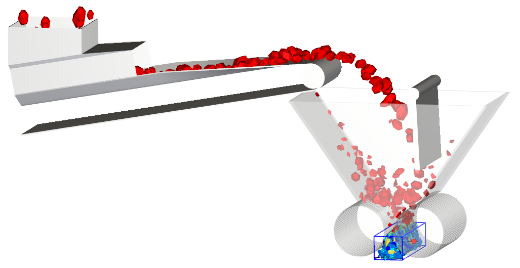
From the Data panel, under User Processes, right-click Particles Time Selection <01>, point to Show in new | Histogram, and then click Particle Size.
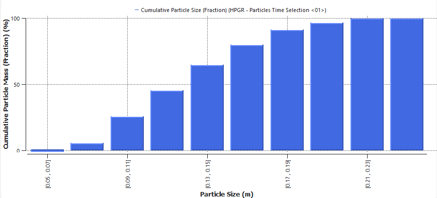
A Histogram window will be created showing the count of particles (and fragments) for each size range that made it into the Cube over the full course of the simulation.
From the upper left corner of the Histogram window, click the Configure histogram icon, and then use the information in the table below to define the settings.
Step Location Parameter or Action Settings A Histogram <01> | Configure Histogram Weight Particle Mass⯆ Cumulative Bins (Enabled) Percent Values (Enabled) Properties Particle Size Limits User Defined⯆ Min 0.05 [m] Max 0.25 [m] Click OK.
The final Histogram shows the cumulative particle (and fragment) size after the original particles go through the rolls.
Note that more than 50% of the particle mass accounted for within the Cube is of a smaller particle size ([0.13, 0.15] (m)) than the smallest particle originally injected (0.15 m).
Because in Part A we enabled the Surface Wear Modification model for the Deflector wall, we are now able to evaluate the results.
Modifications to the geometry can be viewed using the Filter User Process, and then defining Displacement as the Property to analyze. This will show the distance each node was moved.
Use the information in the table below to begin this analysis.
Step Data Entity Editors Location Parameter or Action Settings A Geometries ﹂Deflector
Add a Filter User Process B User Processes ﹂Filter <01>
Property Property Displacement : X⯆ Mode Cut⯆ Type Range⯆ Minimum Value 0.0001 [m] Maximum Value 1 [m] Create or select a 3D View window.
Then, use the information in the table below to change the coloring.
Step Data Entity Editors Location Parameter or Action Settings A User Processes ﹂Filter <01>
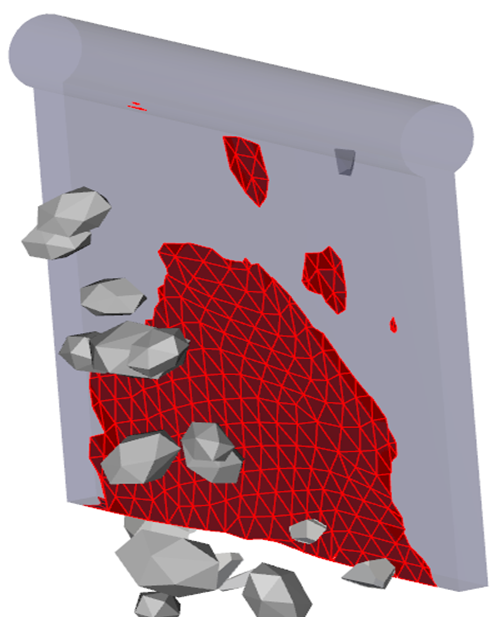
Coloring Transparency (Enabled) Face (Enabled) Face | Property <Solid color>⯆ Face color Dark red Edges (Enabled) Edges | Property <Solid color>⯆ Edge color Red
The results should show only the triangles of the deflector surface that had displacements within the selected displacement range (as shown).
Tip:
Use the Data panel eye icons to hide all but the Deflector Geometry and the Filter <01> User Process.
Use the options on the Time toolbar to view how wear changes over time.
The worn area on the surface of the Deflector geometry can be evaluated using a Time Plot of the Filter <01> User Process you just created.
Use the information in the table below to continue this analysis.
Step Item Editors Location Parameter or Action Settings A Window (menu) Create a New Time Plot B User Processes ﹂Filter <01>
Properties Drag and drop Area : Cell onte the new Time Plot window. C Select the Statistics to Plot (dialog box) Sum (Enabled)
The resulting plot should look similar to the one below.
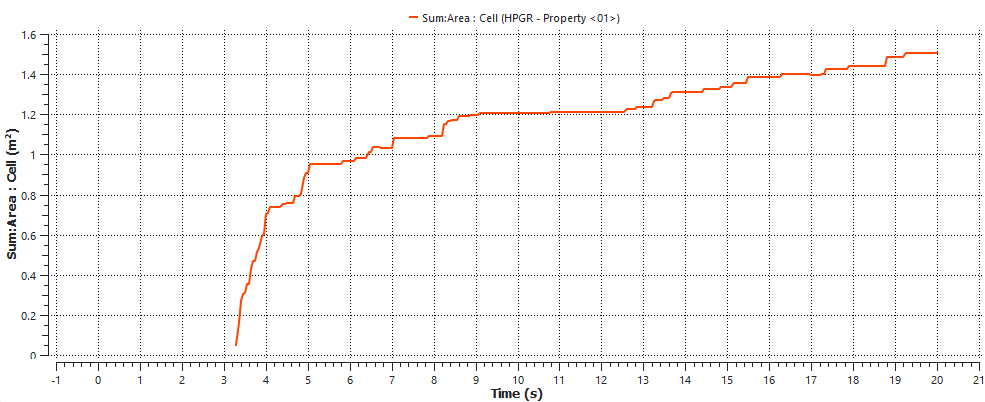
After analyzing the Displacement and Displacement Area, you were able to visualize the affected area on the Geometry Surface and plot this.
Another possible analysis is to verify the Wear Volume Loss that the Geometry suffered. Follow the steps below to visualize the Deflector Geometry's volume loss due to wear and create a Time Plot of the Wear Volume Loss property.
Use the table below to create a color map of the wear volume loss data.
Step Item Editors Location Parameter or Action Settings A Window (menu) Create a New 3D View B Geometries ﹂Deflector
Properties Drag and drop Wear Volume Loss onto the 3D View Window C Color Scales ﹂Wear Volume Loss
Coloring Limits Options User Defined⯆ Limits 0, 0.0001 [m3] Note: Hide every geometry component but the Deflector Geometry.
Under Color Scales select Wear Volume Loss. In the Coloring Tab, click the three dots option to the right of "Color-scale".
You should have the following Color Scale Window open:
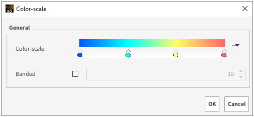
Right-click the blue Mark on the left side of the scale and select grey for the Geometry.
Double-click the scale near the Mark you have just altered to create a new Mark. Drag it to 1% (0.01) and set its color to blue.
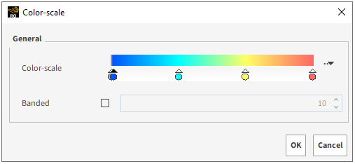
This process allows you to only color the regions that were actually hit by particles, according to its degree of volume loss.
The Image below represents the Deflector Geometry colored by its degree of wear volume loss due to the interaction with particles.
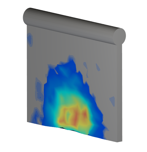
Tip:You can alter the Color Scale Limits and the colors used in the process to perform an analysis to your own liking.
Use the options on the Time toolbar to view how wear changes over time.
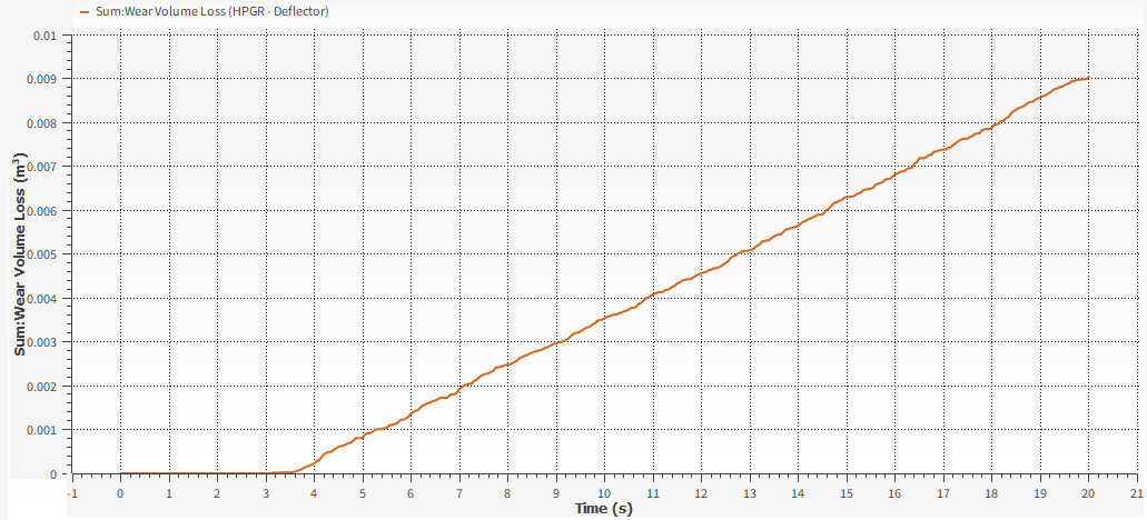
Use the information in the table below to plot the property over time.
Step Item Editors Location Parameter or Action Settings A Window (menu) Create a New Time Plot B Geometries ﹂Deflector
Properties Drag and drop Wear Volume Loss onto the New Time Plot C Select the Statistics to Plot (dialog box) Sum (Enabled) The resulting Plot should look similar to the one below:
You can also analyze wear on the geometries without modifying the surface.
You might recall that in Part A we enabled the Module for Boundary Collision Statistics, and chose to collect Intensities.
Now that we have that data, we can use it to create a color map of the intensities data, such as shear.
Use the table below to create a color map of the Intensity : Shear.
Step Item Editors Location Parameter or Action Settings A Window (menu) Create a New 3D View B Geometries ﹂Deflector
Properties Drag and drop Intensity : Shear onto the 3D View Window C Color Scales ﹂Intensity : Shear
Coloring Limits options User Defined ⯆ Limits 0, 15000 [W/m2] Under Geometries, use the eye icons to hide all but the Deflector component.
The color map should look similar to the image below.
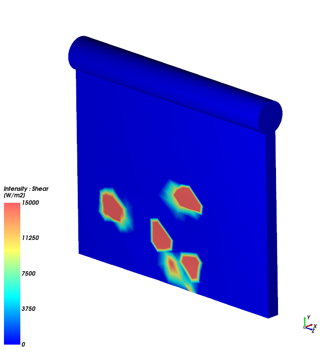
Tip: You can use the Time slider to see how shear intensity changes over time.
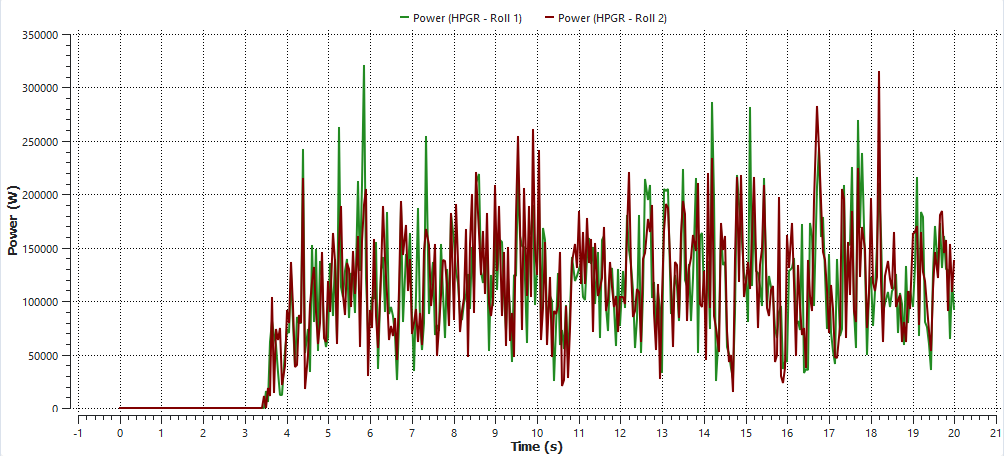
It takes a certain amount of power for the two Roll geometries to successfully comminute the material.
We can use the same Intensities data we chose to collect in Part A to measure the power draw directly from the geometries.
Use the information on the table below to create a Time Plot of the power used for the rolls.
Step Item Editors Location Parameter or Action Settings A Window (menu) Create a New Time Plot B Geometries ﹂Roll 1
Curves Drap and drop Power onto the Time Plot C Geometries ﹂Roll 2
Curves Drap and drop Power onto the Time Plot
The results should look similar to the plot below.
This is a useful way to compare the results with real data and to calibrate the material properties correctly.
This completes Part B of this tutorial.
Rocky was used to study breakage, surface wear, and power draw in an HPGR.
During this tutorial, it was possible to:
Use a Cube and a Particles Time Selection User Process to collect and analyze particles and fragments.
Use a Filter User Process to visualize the surface area displacement.
Use the collected intensities data to view a color map of wear.
Use the Wear Volume Loss property to view a color map of wear.
Use Time Plots and Curves to compare power draw.
What's Next?
If you have completed this tutorial successfully, then you are ready to move on to next tutorial.