


In (Part A), you will create the initial Workbench project, and will set up and run the CFD case using Ansys Fluent.
In (Part B), you will set up and run (without coupling) the DEM portion of the simulation in Rocky.
In (Part C), you will re-run the Rocky case one-way coupled with the results from Ansys Fluent, and will then analyze the coupled simulation results in Rocky.
The main purpose of this tutorial is to use Ansys Workbench to set up and run a CFD case using Ansys Fluent that will be later used in a one-way coupling simulation with Rocky DEM.
Important: Even if you are already familiar with CFD, please follow Part A in order to understand the main limitations and needs for coupling with Rocky.
Part B will cover setting up the Rocky project and running the initial DEM simulation; Part C will cover one-way coupling the DEM project with the CFD results.
The windshifter scenario considered in this tutorial evaluates how air flowing upwards through a pipe affects the different materials that discharge into it.
In this tutorial, you will learn how to:
Verify and install Ansys coupling components within Rocky
Create a project in Ansys Workbench
Import a geometry into Ansys Discovery
Set up a CFD case in Ansys Fluent
To complete this tutorial, you are required to have on a Windows machine the following:
(1) A valid license for the following Ansys products: Ansys Discovery, Ansys Rocky and Ansys Workbench 2025 R2.
Important: This ADVANCED tutorial assumes that you are already familiar the the following programs and resources:
The Ansys Workbench platform
Note: Ansys Rocky and Ansys Workbench integration is currently supported only on Windows.
The Ansys Discovery program
The Ansys Fluent program and project workflow
If you are not familiar with these programs, please refer to the Ansys user documentation for introduction and usage instructions before beginning this tutorial.
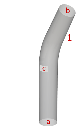
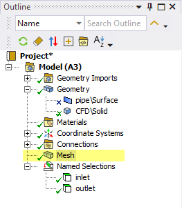
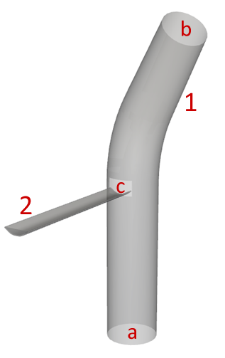
The geometry for Part A of this tutorial includes the following component:
(1) pipe, which itself has the following regions:
(a) inlet (fluid flow)
(b) outlet (fluid flow)
(c) opening (material flow)
In the tutorial directory the .dsco file for the pipe geometry can be found.
To begin setting up the tutorial:
Download the
dem_tut13_files.zipfile here .Unzip
dem_tut13_files.zipto your working directory.Open Ansys Workbench 2025 R2 (or other supported version).
Save the empty Workbench Project from the File, Save As... menu item.
Tip: If you run into settings or procedures in these tables that you are not yet familiar with, please refer to the Rocky User Manual and/or other Tutorials (via the Introductory Tutorials and Advanced Tutorials) to find the detailed instructions you need.
Next, we'll add the Fluent component to the Workbench project, import geometry into the Fluent component, and then set the parameters for the Fluent mesh. Follow the steps:
From the Toolbox panel, under Analysis Systems, drag and drop Fluid Flow (Fluent) onto the Project Schematic.
On the Fluid Flow (Fluent) block, right-click Geometry, point to Import Geometry, and then click Browse....
From the dialog that appears, locate the geometry folder inside the dem_tut13_files folder you downloaded, select the input file tutorial_13_geometry.dsco, and then click Open.
Tip: The Geometry will show a green checkmark if the .dsco file is correctly imported.
Note: Although we will import the same geometry file into Ansys Rocky and Ansys Fluent, they cannot share the same geometry component within the Ansys Workbench project. This is because the solid body used for Fluent meshing needs to be supressed in Rocky.
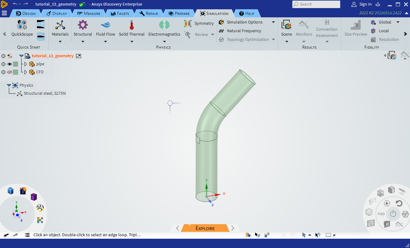
From the Fluid Flow (Fluent) block, double-click the Mesh component. Meshing software automatically opens with the linked geometry already imported.
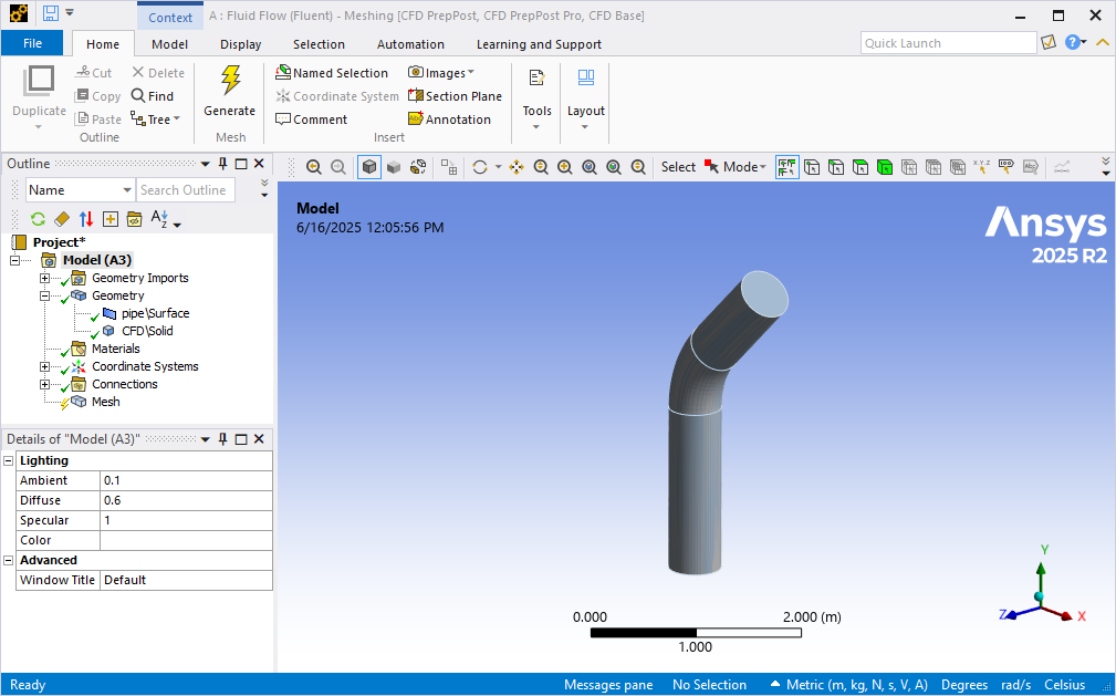
From the Outline panel, under Model | Geometry, right-click pipe\Surface, and then click Suppress Body.

Define the inlet and outlet boundary conditions by creating two Named Selections as follows:
In the main view, using the face selection tool, select the lower face of the pipe, and then do the following:

Right-click this selection and then click Create Named Selection....
Define the Name as "inlet", and then click OK.
Select the upper face of the pipe, and then do the following:
Right-click this selection and then click Create Named Selection....
Define the Name as "outlet", and then click OK.
You should now have two entries under Named Selections (as shown).

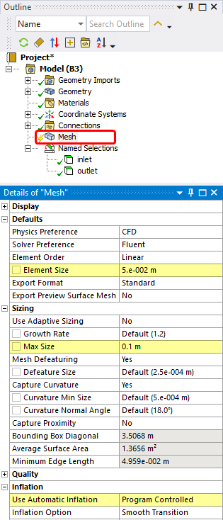
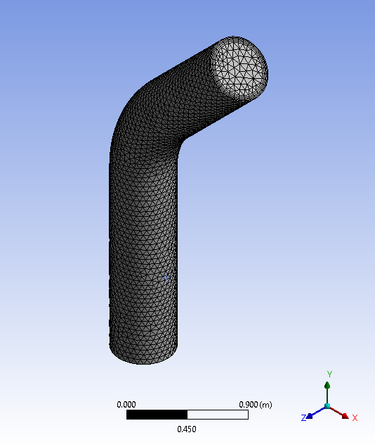
Under Model, click Mesh.
From the Details of "Mesh" panel, define (as shown):
Under Defaults, the Element Size.
Under Sizing, the Max Size.
Under Inflation, the Use Automatic Inflation parameter.
From the Outline panel, right-click Mesh and then click Generate Mesh.
Right-click Mesh again, and then select Update (this will export the mesh to Fluent).
The mesh for the CFD analysis is now ready.
Close the Meshing program and return to Workbench.
Save your Workbench project.
Let's set up the Fluent portion of our project:
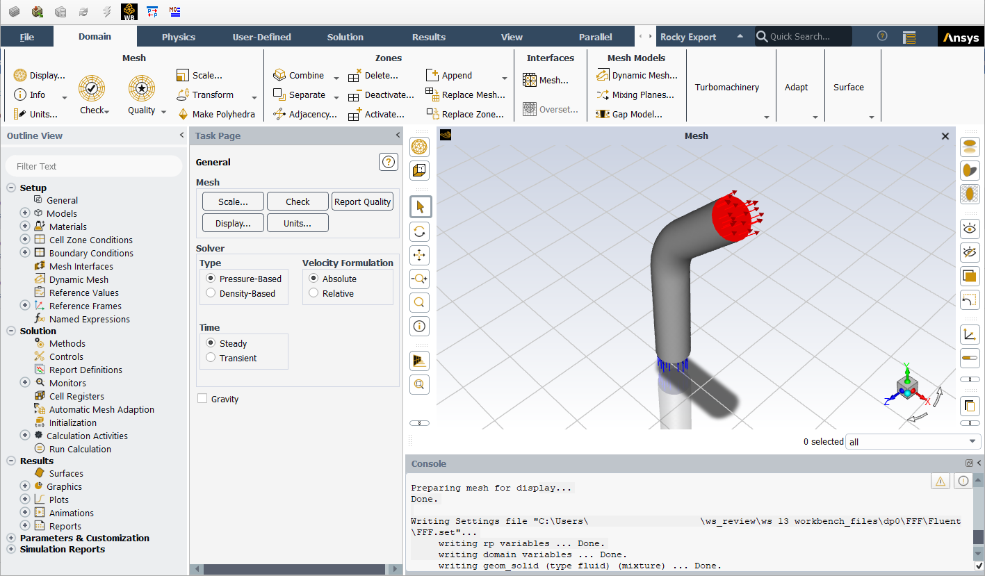
From the Fluid Flow (Fluent) block, double-click the Setup component.
From the Fluent Launcher dialog that appears, select Double Precision (as shown), ensure 3D is selected for Dimension, and then click Start.
Important: Double Precision and 3D are required for coupling with Rocky.
Note: Fluent allows parallel processing, which means that separate solver resources can be used for Fluent. If you want to enable this feature, under Parallel (Local Machine), define the Solver Processes or Solver GPUs you want Fluent to make use of.

Ansys Fluent will open with a new project and the meshed geometry already imported.
Then, define the Model settings:
From the Outline View tree panel, under Setup | Models, double-click Viscous.

On the Viscous Model dialog, under Model, select k-epsilon (2 eqn).
Under Near-Wall Treatment, select Scalable Wall Functions.
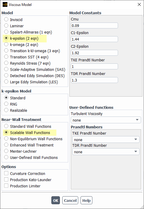
Click OK.
Later in this tutorial, we will run the one-way coupled case with the Thermal Model enabled in Rocky.
To enable thermal properties for the fluids, do the following:
From the Outline View tree panel, under Setup | Models, double-click Energy.

From the Energy dialog, enable the Energy Equation checkbox (as shown).
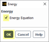
Click OK.
Next, we need to define both the Specific Heat and Thermal Conductivity for the fluid.
Note: In this version of Rocky, both constant and polynomial thermal properties for fluid materials are supported.
In this tutorial, we want constant values set for the fluid thermal properties. Let's verify:
From the Outline View tree panel, under Setup | Materials | Fluid, double-click air.
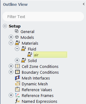
From the Create/Edit Materials dialog, verify that both Cp (Specific Heat) and Thermal Conductivity are defined as constant.

Click Close (no changes).
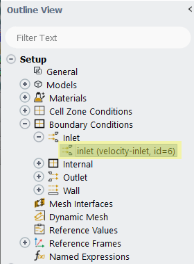
Next, let's define the boundary conditions:
From the Outline View tree panel, under Setup | Boundary Conditions |Inlet, double-click inlet (velocity-inlet, id=6).
From the Velocity Inlet dialog, on the Momentum tab, define the Velocity Magnitude (as shown).

On the Thermal tab, define the Temperature (as shown).
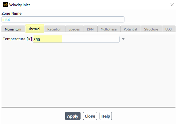
Click Apply and then click Close.
To initialize the Fluent case, do the following:
From the Outline View tree panel, under Solution, double-click Initialization.
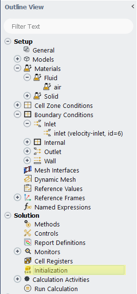
From the Task Page, click Initialize (as shown).
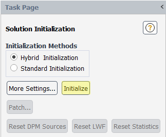
Finally, solve the Fluid case by doing the following:
From the Outline View tree panel, under Solution, double-click Run Calculation.

From the Run Calculation Task Page, define the Number of Iterations (as shown), and then click Calculate.
The Scaled Residuals window appears (as shown).

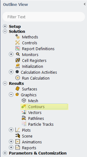
Once the calculation is finished and the fluid results are available, it is possible to analyze the fluid flow.
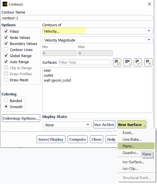
From the Outline View tree panel, under Results | Graphics, right-click Contours, and then click New.
From the Contours dialog, define Contours of (as shown).
From the New Surface list, click Plane....
On the Plane Surface dialog, do all of the following:
Define the New Surface Name (as shown).
Under Method, select Point and Normal (as shown).
Under both Point and Normal, define the x, y, and z values (as shown), and then click Create.
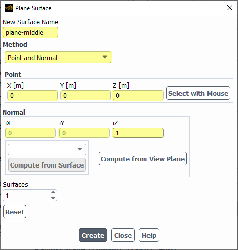
Click Close.
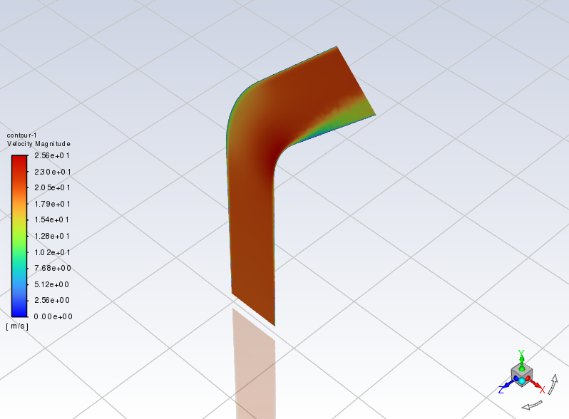
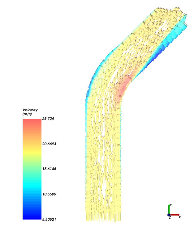
From the Contours dialog, select only the new plane-middle surface, and then click Save/Display.
The results are shown on below.
Close the Contours dialog.
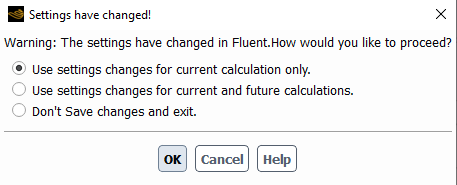
Close Fluent and return to Workbench.
Tip: If you get a Settings have changed! message at this point, you can select either of the first two options (as shown), and then click OK.
Save the Workbench project.
This completes Part A of this tutorial.
For more information about setting up a Fluent case for one-way coupling with Rocky, we suggest referencing the Rocky CFD Coupling Technical Manual.
To access it, from the main Rocky Toolbar click Help, point to Manuals, and then click CFD Coupling Technical Manual.
For further information about any of the Ansys products used in this tutorial, please refer to your Ansys user documentation.
Through Ansys Workbench, Ansys Fluent was used to set up and run a CFD simulation that will later be one-way coupled with Rocky.
During this tutorial, it was possible to:
Create a new Ansys Workbench project.
Use Ansys Meshing to generate the geometry's mesh.
Use Ansys Fluent to set up a CFD case.
What's Next? If you completed this part successfully, then you are ready to move on to Part B and create the Rocky project that will later be one-way coupled with this CFD case.
The main purpose of this tutorial is to use Ansys Workbench to set up and run a DEM case using Rocky that will later be one-way coupled with the Fluent case we created in Part A.
Part C will cover one-way coupling the DEM project with the CFD results.
As a reminder, the windshifter scenario considered in this tutorial evaluates how air flowing upwards through a pipe affects the different materials that discharge into it.
You will learn how to:
Prepare a geometry using Discovery via Workbench
Open Rocky through Workbench
Enable a thermal model
Collect particle-fluid statistics
Use Equivalent Sphere Diameter to specify particle size
Set up and run a DEM case (without coupling)
Delete results within a Rocky project
And you will use these features:
Thermal Modeling
CFD Coupling Particle Statistics
Particle Size Type
Continuous Injection Input
Coloring by Property
To complete this tutorial, you are required to have on a Windows machine the following:
(1) A valid license for the following Ansys products: Discovery, Rocky and Workbench 2025 R2.
Important: This ADVANCED tutorial assumes that you are already familiar the the following programs and resources:
The Ansys Workbench platform.
If that is not the case, please refer to the Ansys Workbench user documentation for basic introduction about Workbench usage before beginning this tutorial.
Note: Rocky and Ansys Workbench integration is currently supported only on Windows.
The Rocky user interface (UI) and the Rocky project workflow.
If this is not the case, it is recommended that you complete at least Tutorials 01- 05 before beginning this tutorial.
The geometries for Part B of this tutorial includes:
(1) pipe, which itself includes the following regions:
(a) inlet (fluid flow)
(b) outlet (fluid flow)
(c) opening (material flow)
(2) Receiving Conveyor
The pipe will be imported from the Workbench project.
The Receiving Conveyor will be created in Rocky.
If you completed Part A of this tutorial, ensure that the Ansys Workbench project you created is open. (Part B will continue from where Part A left off.)
If you did not complete Part A, do all of the following:
Download the
dem_tut13_files.zipfile here .Unzip
dem_tut13_files.zipto your working directory.Open Ansys Workbench.
Important: To make use of the Workbench project file provided, you must have Ansys Workbench 2025 R2. If you have an earlier software version, please upgrade it or complete Part A from scratch.
From the Workbench program, click the Open Project button, find the dem_tut13_files folder, and then from the tutorial_13_A_processing-fluent folder, open the tutorial_13_A_processing-fluent.wbpj file.
With the project open in Workbench, you are now ready to begin Part B.
In Workbench, add the Rocky component as follows:
From the Toolbox panel, under the Analysis Systems item, drag and drop Particle Dynamics (Rocky) onto the Project Schematic.
From the Workbench File menu, click Save As.
From the dialog that appears, select a file location, define the File Name for the Workbench project as tutorial_13_B-processing-rocky.wbpj, and then click Save.
Tip: If you run into settings or procedures in these tables that you are not yet familiar with, please refer to the Rocky User Manual and/or other Tutorials (via the Introductory Tutorials and Advanced Tutorials) to find the detailed instructions you need.
Next, let's prepare the geometry for Ansys Rocky using Ansys Discovery via Ansys Workbench:
Important: As stated before, we now have to prepare the geometry that will be used in Rocky, removing the solid region that accounts for the interior of the pipe, which was used in the Fluent meshing. In Rocky, this geometry component would occupy the interior of the pipe, making it impossible for us to analyze the interaction between particles and fluid.
On the Particle Dynamics (Rocky) block, right-click Geometry, point to Import Geometry, and then click Browse....
From the dialog that appears, locate the geometry folder inside the dem_tut13_files folder you downloaded, select the input file tutorial_13_geometry.dsco, and then click Open.
Tip: The Geometry will show a green checkmark if the .dsco file is correctly imported.
To prepare the Geometry for later coupling between Rocky and Fluent, do the following:
On the Geometry block, right-click Geometry and select Edit Geometry in Discovery....
Ansys Discovery opens with the linked geometry already imported (as shown).
The geometry is composed of a solid (fluid volume for CFD) and a surface (walls for DEM).
For this tutorial, we want Rocky to import only the Surface of the geometry, as this is the only part that will be interacting with the particles.
Important: Rocky only imports components that are not excluded from simulation.
From the Structure tree, check if the Solid component is excluded from the simulation (as shown).
Close Discovery and return to Workbench.
Save the Workbench Project.

Important: Ensure Rocky is closed before you begin.
Next, let's define the Rocky project through Workbench.
From the Workbench project's Rocky block, double-click the Setup component.
The Rocky program opens automatically with a connected project that has the pipe geometry ("pipe") already included.
From the Rocky Menu, go to Options | Ansys and select Install Fluent/Rocky export.
Important: This step is necessary for Rocky to obtain Fluent information when running the coupled simulation later.
Now that Rocky is open, we can begin setting up our DEM project.
For the Physics step, we will enable thermal.
For the Modules step, we will be turning on the collection of CFD Coupling Particle Statistics.
This module collects particle-fluid interactions for later post-processing.
For this tutorial, we are primarily interested in collecting the drag-related data.
Use the information in the table below to begin setting up your Rocky project.
Step Data Entity Editors Location Parameter or Action Settings A Physics Thermal Enable Thermal (Enabled) B Modules Modules CFD Coupling Particle Statistics (Enabled) C Modules ﹂CFD Coupling Particle Statistics
CFD Coupling Particle Statistics Drag Force (Enabled) Tip: If you run into settings or procedures in these tables that you are not yet familiar with, please refer to the Rocky User Manual and/or other Tutorials (via the Introductory Tutorials and Advanced Tutorials) to find the detailed instructions you need.
For this tutorial, a Receiving Conveyor will be created to transport the material to the pipe.
From the Data panel, right-click Geometries, point to Conveyor Templates and then select Create Receiving Conveyor.
A new geometry component will appear.
Select the newly added Receiving Conveyor <01> component.
Step Data Entity Editors Location Parameter or Action Settings A Geometries ﹂Receiving Conveyor <01>
Receiving Conveyor | Geometry Length 1.5 [m] Belt Width 0.25 [m] Triangle Size 0.01 [m] Belt Thickness 0.01 [m] … | Orientation Vertical Offset 1.5 [m] Horizontal Offset -1.7125 [m] … | Belt Profile Lower Corner Radius 0.1 [m] … | Belt Motion Belt Speed 1 [m/s] Step Data Entity Editors Location Parameter or Action Settings A Geometries Create Rectangular Surface B Geometries ﹂Rectangular Surface <01>
Rectangular Surface Center Coordinates -1.55, 1.7, 0 [m] Length 0.3 [m] Width 0.15 [m] Orientation | Angle 30 [dega] Orientation | Angle 0, 0, 1 [ - ]
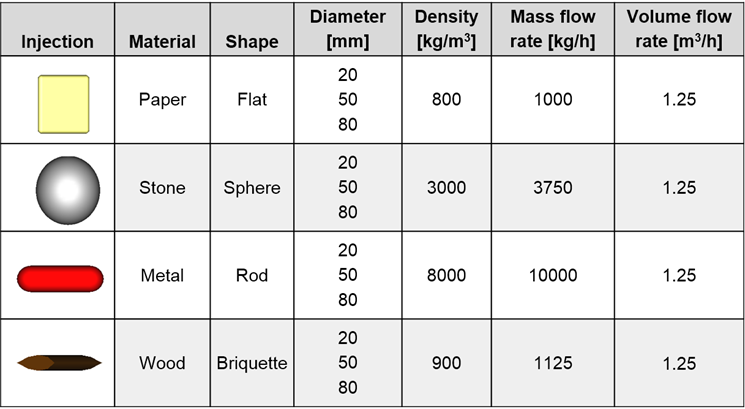
For this tutorial, we want four particle groups, each with different material characteristics, but with the same particle size distribution (PSD) and the same volume flow rates in each group.
In this way, we can later verify how the drag force computed using a drag law that takes into account shape and orientation will act on these particles depending on the particle density and volume.
For the Materials step, we will use Default Particles to define four new materials.
From the Data panel, under Materials, right-click Default Particles, and then click Duplicate.
Repeat this process until you have 3 new entries for Materials.
Use the information in the tables that follow to define each of these four materials.
Step Data Entity Editors Location Parameter or Action Settings A Materials ﹂Default Particles
Material Name Metal Use Bulk Density (Cleared) Density 8000 [kg/m3] Thermal Conductivity 80 [W/m.K] Specific Heat 400 [J/kg.K] B Materials ﹂Default Particles <01>
Material Name Paper Use Bulk Density (Cleared) Density 800 [kg/m3] Thermal Conductivity 0.05 [W/m.K] Specific Heat 2000 [J/kg.K] C Materials ﹂Default Particles <02>
Material Name Stone Use Bulk Density (Cleared) Density 3000 [kg/m3] Thermal Conductivity 3 [W/m.K] Specific Heat 840 [J/kg.K] D Materials ﹂Default Particles <03>
Material Name Wood Use Bulk Density (Cleared) Density 900 [kg/m3] Specific Heat 2000 [J/kg.K]
For the Particles step, we will be creating four separate particle groups corresponding to the four different materials we have defined.
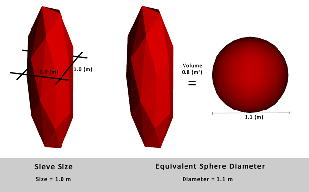
In this tutorial, we want all these groups to have the same PSD.
To accomplish this, we'll be using the Equivalent Sphere Diameter Size Type.
This option is especially useful for irregular objects, as it allows the particle size to be based upon the diameter of a sphere with equivalent volume.
Use the information in the tables that follow to define each of these four particle shapes.
Step Data Entity Editors Location Parameter or Action Settings A Particles Create Particle B Particles ﹂Particle <01>
Particle Name Metal Shape Sphero-Cylinder ⯆ Material Metal ⯆ C Particles ﹂Metal
Particle | Size Size Type Equivalent Sphere Diameter Add row (x2) (1) Diameter | Cumulative % 0.08 [m] @ 100 [%] (2) Diameter | Cumulative % 0.05 [m] @ 40 [%] (3) Diameter | Cumulative % 0.02 [m] @ 10 [%] … | Shape Vertical Aspect Ratio 3.00 [ - ] D Particles ﹂Metal
Duplicate E Particles Metal <01>
Particle Name Paper Shape Sphero-Polygon ⯆ Material Paper ⯆ … | Shape Vertical Aspect Ratio 1.00 [ - ] Horizontal Aspect Ratio 0.10 [ - ] Number of Corners 4 [ - ] F Particles ﹂Paper
Duplicate G Particles ﹂Paper <01>
Particle Name Stone Shape Sphere ⯆ Material Stone ⯆ H Particles ﹂Stone
Duplicate I Particles ﹂Stone <01>
Particle Name Wood Shape Briquette ⯆ Material Wood ⯆ … | Shape Vertical Aspect Ratio 0.30 [ - ] Side Angle 30.00 [ - ] Number of Corners 16 [ - ]
For the Inlets and Outlets step, we will create one Particle Inlet to release from Rectangular Surface <01> all four of the particle groups we just defined.
Specifically:
Each particle group will be given a mass flow rate that, along with the material density, will help us reach our goal of achieving the same volume flow rate per group.
We will also be prescribing these particle groups with the same initial temperature.
Use the information in the table that follows to define your Inputs.
Step Data Entity Editors Location Parameter or Action Settings A Inlets and Outlets Create Particle Inlet B Inputs ﹂Particle Inlet <01>
Particle Inlet Entry Point Rectangular Surface <01> ⯆ Particle Inlet | Particles Add row (x4) (1) Particle | Mass Flow Rate | Temperature Metal ⯆ @ 240 [t/d] 25 [degC] (2) ... Paper ⯆ @ 24 [t/d] 25 [degC] (3) ... Stone ⯆ @ 90 [t/d] 25 [degC] (4) ... Wood ⯆ @ 27 [t/d] 25 [degC]
For illustration purposes, we will first run the case without fluid flow.
Use the information in the table that follows to finish setting up your Rocky project.
Step Data Entity Editors Location Parameter or Action Settings A Solver Solver | Time Simulation Duration 5 [s] Solver | General Simulation Target CPU ⯆
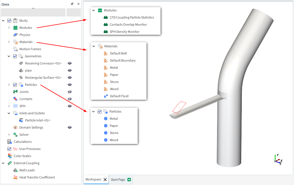
With a 3D View window opened, your Data panel and Workspace should look similar to the image shown below.
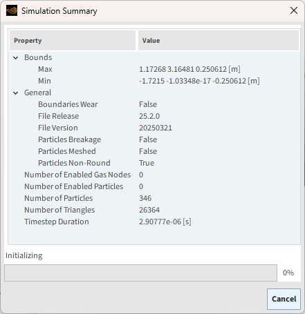
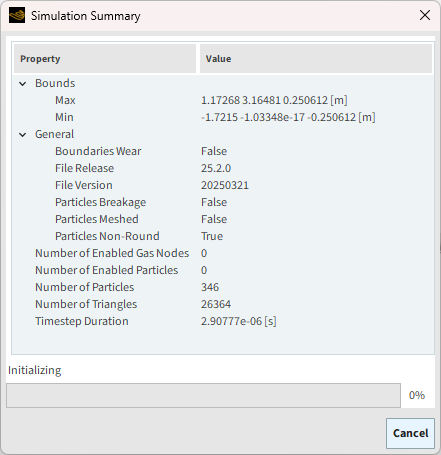
From the Solver entity, click Start.
The Simulation Summary screen appears (as shown), then processing begins.
Tip: You can use the Auto Refresh checkbox to view in a 3D View window the results during processing.
Note: When the simulation processing is done inside Workbench—as is done in this Tutorial—all files are saved in the Workbench file directory, including the ones needed for Rocky.
After Rocky is finished processing, you may post-process the (pre-fluid) particle-only results.
Because as of yet, there is still no fluid coupling, we are able to analyze only the particle behavior at this point.
Doing so now can later help us see the changes in behavior once fluid effects are applied (in Part C).
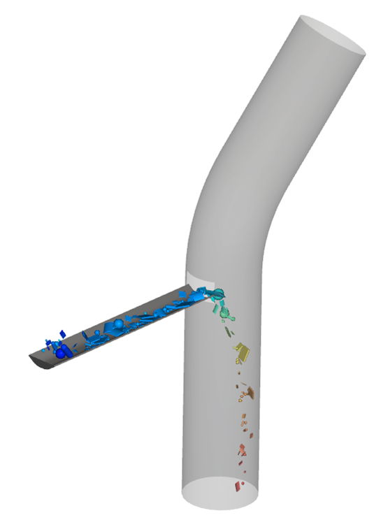
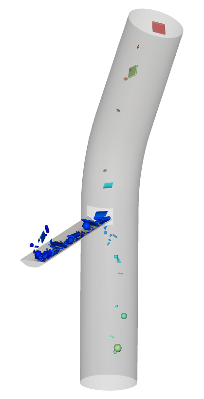
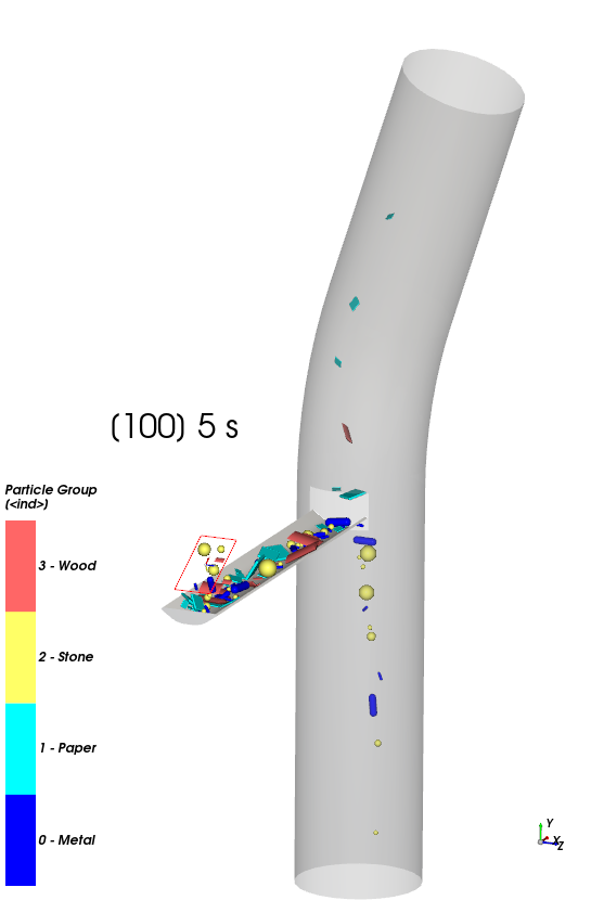
Let's start by looking at particle trajectory through the pipe.
Select or create a 3D View window.
Use the information in the table below to define what is shown in this window.
Step Data Entity Editors Location Parameter or Action Settings A Particles Coloring Nodes (Enabled) Nodes | Property Particle Group ⯆ B Geometries ﹂Design1
Coloring Transparency (Enabled) Use the options on the Time toolbar to see the particles' trajectory through the pipe.

Notice that without fluid effects, all particle groups fall downwards through the pipe.
At the final timestep (5 s), save a copy of this image by right-clicking within the 3D View window, and then clicking Save Image.
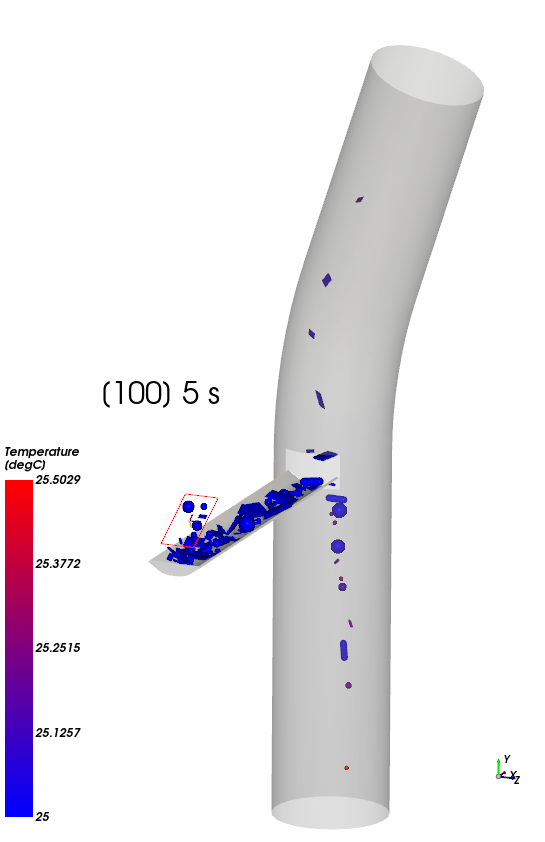
Now, let's look at temperature.
Use the information in the table below to re-define what is shown in the 3D View window.
Step Data Entity Editors Location Parameter or Action Settings A Particles Coloring Nodes | Property Temperature ⯆ B Color Scales ﹂Temperature
Coloring Limit options Automatic PER View ⯆ 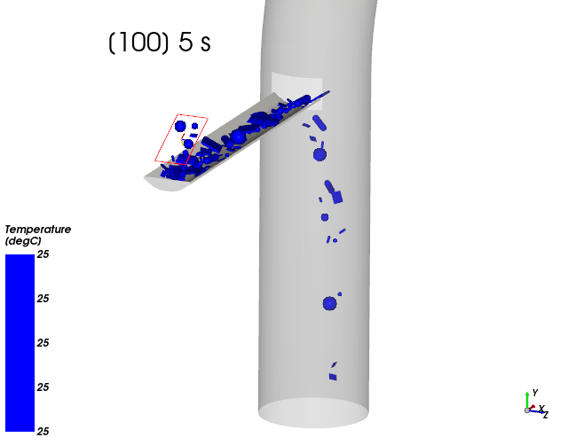
Notice that even over time, without fluid effects, all particles maintain their same initial temperature.
At the final timestep (5 s), save a copy of this image by right-clicking within the 3D View window, and then clicking Save Image.
Now that we have analyzed the particle flow without the effects of fluids, let's have Rocky delete the simulation results so that we can re-run them (through Workbench) with the fluid results included.
An easy way to delete the results in Rocky is to use the Clear Results button.
From the Simulation toolbar, select the Clear Results button.
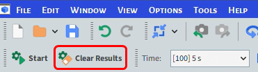
A Dialog will appear asking whether you want to delete the results. Click Yes to delete the results.
Save and Close Rocky and return to Workbench.
Save the Workbench project.
This completes Part B of this tutorial, in which Ansys Workbench was used to set up and run an initial Rocky simulation that will later be one-way coupled with the CFD results we created in Part A.
During this tutorial, it was possible to:
Set up and run the initial Rocky simulation through Workbench.
Verify that Rocky is ready for coupling with Ansys.
Import and edit a geometry into Workbench using Ansys Discovery.
Analyze the (pre-fluid) behavior of the particle flow through the pipe.
Delete the DEM results to reset the Rocky project back to just the setup portion.
What's Next? If you completed this tutorial successfully, then you are ready to move on to Part C and use Workbench to one-way couple the CFD results with this Rocky project.
The main purposes of this tutorial are to use Ansys Workbench to run a one-way coupled DEM-CFD simulation using Ansys Rocky and Ansys Fluent, and then analyze those results.
We will make use of the CFD results we obtained in Part A and the Rocky project setup we created in Part B.
As a reminder, the windshifter scenario considered in this tutorial evaluates how air flowing upwards through a pipe affects the different materials that discharge into it.
You will learn how to:
Create the link between Rocky and Fluent in Workbench
Set up the fluid forces models in Rocky
View a slice of the fluid vectors
Process a one-way coupled simulation
Analyze particle flow, drag, and temperature
And you will use these features:
1-Way Fluent CFD Coupling
Cube User Process
Coloring Vectors by Property
Coloring Nodes by Property
To complete this tutorial, you are required to have on a Windows machine the following:
(1) A valid license for the following Ansys products: Discovery, Rocky and Workbench 2025 R2.
Important: This ADVANCED tutorial assumes that you are already familiar the following programs and resources:
The Ansys Workbench platform.
If that is not the case, please refer to the Ansys Workbench user documentation for basic introduction about Workbench usage before beginning this tutorial.
Note: Rocky and Ansys Workbench integration is currently supported only on Windows.
The Rocky user interface (UI) and the Rocky project workflow.
If this is not the case, it is recommended that you complete at least Tutorials 01- 05 before beginning this tutorial.

As a reminder, the geometry for Part C of this tutorial is composed of:
(1) pipe, which itself has the following regions:
(a) inlet (fluid flow)
(b) outlet (fluid flow)
(c) opening (material flow)
(2) Receiving Conveyor
Note: These components were added in Part A and Part B of this tutorial.
If you completed Part B of this tutorial, ensure that the Ansys Workbench project you last saved is open. (Part C will continue from where Part B left off.)
If you did not complete Part B, do all of the following:
Download the
dem_tut13_files.zipfile here .Unzip
dem_tut13_files.zipto your working directory.Open Ansys Workbench.
Important: To make use of the Workbench project file provided, you must have Ansys 2025 R2 or later and Rocky 2025 R2 or later. If you have an earlier version of either of these programs, please upgrade to the latest version of Rocky and the latest version of Ansys that is supported by Rocky, or complete Parts A and B from scratch.
From the Workbench program, click the Open Project button, find the dem_tut13_files folder, and then from the tutorial_13_B_processing-rocky folder, open the tutorial_13_B_processing-rocky.wbpj file.
With the project open in Workbench, you are now ready to begin Part C.
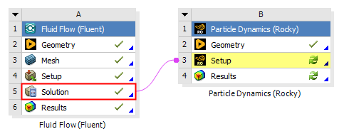
Let's start by connecting the Fluent results with Rocky in Workbench.
From the Fluid Flow (Fluent) component, right-click Solution and select Refresh.
From the Fluid Flow (Fluent) component, right-click Solution and select Update.
From the Fluid Flow (Fluent) component, right-click Results and select Refresh.
From the Project Schematic, drag and drop the Solution component from the Fluid Flow (Fluent) block onto the Setup component of the Rocky block (as shown).
Note: This action will automatically generate a link between the CFD results and the Rocky project.
From the Rocky block, double-click the Setup component.
Due to the link created in Workbench, the Rocky project opens with CFD results automatically included.
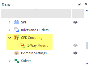
Define the CFD Coupling options in Rocky:
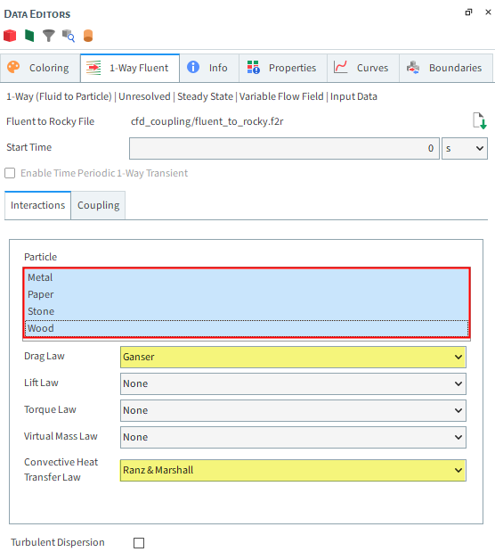
From the Data panel, under CFD Coupling, select 1-Way Fluent.
From the Data Editors panel, select the 1-Way Fluent | Interactions tab, and then from the Particle list, multi-select all four of the particle groups listed (as shown).
Define the Drag Law.
Note: This drag law was selected because it is suitable for both spherical and non-spherical particles.
Also define the Convective Heat Transfer Law (as shown).
Now that the CFD results are within Rocky, you can visualize the nodes of the cell centroids making up the Fluent mesh.
Important: Given the amount of elements, showing all vectors for your CFD meshes is not considered good practice as it can freeze the Rocky interface.
A better practice is to create a thin slice of your mesh and show only the vectors within that slice. We will start by creating a Cube.
Use the information in the below table to begin creating this view.
Step Data Entity Editors Location Parameter or Action Settings A CFD Coupling ﹂ 1-Way Fluent
Create a Cube User Process B User Processes ﹂Cube <01>
Cube Center 0.4, 1.5, 0 [m] Magnitude 1.4, 3, 0.02 [m] From the Data panel, under User Processes, right click the Cube <01> entry, point to Show in new, and then click 3D View.
With the new 3D View window selected, hide all the geometry components and Particles by clicking the eye icon to the right of the entries on the Data panel so that the icon appears closed.
Use the information in the table below to finish setting up the view.
Step Data Entity Editors Location Parameter or Action Settings A User Processes ﹂Cube <01>
Coloring Vectors (Enabled) Vectors | Property Velocity ⯆ Vectors | Vector scale 0.2 [ - ] Vectors | Normalized Vectors (Enabled)
The colored vectors within the slice of pipe indicate that the fluid moves up and around the bend of the pipe.
As the previous iteration did not include CFD results, it is necessary to run the simulation again to calculate how the fluid flow affects the particles.
Use the information in the table below to ensure your solver parameters are correct.
Note: The parameters are the same ones we defined earlier in Part B to simulate only particles, so you shouldn't have to make any changes for this step.
Step Data Entity Editors Location Parameter or Action Settings A Solver Solver | Time Simulation Duration 5 [s] Solver | General Simulation Target CPU ⯆ Click Start.
The Simulation Summary screen appears (as shown), then processing begins.
Tip: You can use the Auto Refresh checkbox to view in a 3D View window the results during processing.
Note: When the simulation processing is done inside Workbench, as shown in this tutorial, all files are saved in the Workbench file directory, including the ones needed for Rocky.
After the simulation is done processing, you can analyze the coupled particle-fluid flow that was simulated, and compare it to the particle-only flow we analyzed in Part B.
With a 3D View window selected, use the information in the table below to define what is shown in the window.
Tip: Both particles and geometries will be analyzed in this comparison. Use the eye icons on the Data panel to show the related entities if they are hidden.
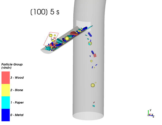
Step Data Entity Editors Location Parameter or Action Settings A Particles Coloring Nodes (Enabled) Nodes | Property Particle Group ⯆ B Geometries ﹂Design1
Coloring Transparency (Enabled) Use the options on the Time toolbar to view the particles' trajectory over time.
At the final timestep (5 s), compare these particle-fluid results (on the right) with the image you took of the particle-only flow in Part B (on the left).
In the particle-fluid simulation (on the right), the lighter Wood and Paper particles are carried up the pipe due to the fluid flow.
Take note of the Particle Group number shown on the color scale. We will need the values for Metal (shown here as 0) and Stone (shown here as 2) later in this tutorial.
A similar comparison can be made with Temperature.
Use the information in the table below to re-define what is shown in the 3D View window.
Step Data Entity Editors Location Parameter or Action Settings A Particles Coloring Nodes | Property Temperature ⯆ B Color Scales ﹂Temperature
Coloring Limit Options Automatic PER View ⯆ Use the options on the Time toolbar to view how the particles' temperature changes over time.
At the final timestep (5 s), compare these particle-fluid results (right) with the image you took of the particle-only flow in Part B (left).

In the particle-fluid simulation (right), heat is transferred from the fluid to the particles.
Note: Particles reach different temperatures due to the different combinations of heat capacity, conductivity and surface area.
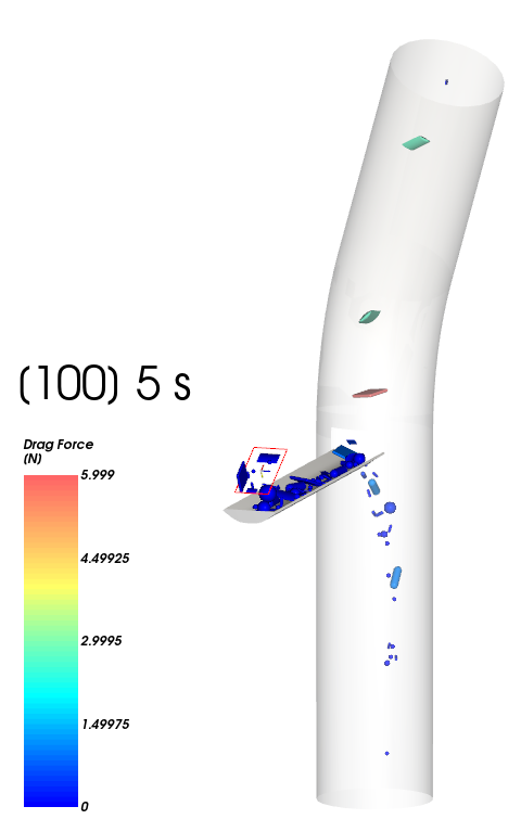
Earlier in Part B of this tutorial, we turned on the CFD Coupling Particle Statistics module, and chose to collect data on Drag Force.
We can now evaluate how the drag force affects the particles.
With a 3D View window selected, use the information in the table below to define what is shown.
Step Data Entity Editors Location Parameter or Action Settings A Particles Coloring Nodes (Enabled) Nodes | Property Force: Drag ⯆ Use the Time toolbar to see how drag affects the particles over time.
We can further evaluate the drag force by comparing its effects on different groups of particles.
Enable the Expressions/Variables panel (from Menu | Tools).
Follow the steps in the table below to filter the Metal particle group into a specific size range.
Step Data Entity Editors Location Parameter or Action Settings A Particles Create a Cube User Process B User Processes ﹂Cube <02>
Cube Center 0, 1.4, 0 [m] Magnitude 0.5, 0.5, 0.5 [m] C User Processes ﹂Cube <02>
Create a Particles Time Selection User Process D User Processes ﹂Particles Time Selection <01>
Time Selection | Time Range Filter Domain Range All ⯆ E User Processes ﹂Particles Time Selection <01>
Create a Filter User Process F User Processes ﹂Filter <01>
Filter Name All Smalls Property Particle Equivalent Diameter ⯆ Type Range ⯆ Minimum Value 0.02 [m] Maximum Value 0.03 [m] Follow the steps in the table below to filter the Stone particle group into a specific size range and then compare the resulting drag forces
Step Data Entity Editors Location Parameter or Action Settings G User Processes ﹂All Smalls
Create a Filter User Process H User Processes ﹂Filter <01>
Filter Name Metal Smalls Property Particle Group ⯆ Type Value ⯆ Cut value 0 Properties | Force: Drag Drag and drop to Expressions/Variables | Output I User Processes ﹂All Smalls
Create a Filter User Process J User Processes ﹂Filter <01>
Filter Name Stone Smalls Property Particle Group ⯆ Type Value ⯆ Cut Value 2 Properties | Force : Drag Drag and drop to Expressions/Variables | Output Note: For steps H and J, ensure that what you enter for Cut value corresponds to the correct Particle Group number displayed on the color scale within your own project (see 3).
At this point, we have successfully filtered the particles that we want to evaluate drag forces by both size (only the smallest) and group (only Metal and Stone).
Tip:
To better visualize the particles we are analyzing, use the eye icons on the Data panel to hide Particles and every entity under User Processes except the Metal Smalls and Stone Smalls entities.
Refer to Tutorial 03 - Vibrating Screen for an introduction about Particles Time Selection if you are not familiar with it.
You can also color each property by Particle Group to better differentiate between the metal and stone.
Use the table below to configure the output variables you just created.
Step Item Parameter or Action Settings A Expressions/Variables | Output ﹂Force_Drag
Edit (button) B Edit Properties (dialog box) Name Force_Drag_Metal Property to Curve average ⯆ C Expressions/Variables | Output ﹂Force_Drag_0
Edit (button) D Edit Properties (dialog box) Name Force_Drag_Stone Property to Curve average ⯆
Now you have the average values of the drag forces that acted on the Metal and Stone particles (as shown).
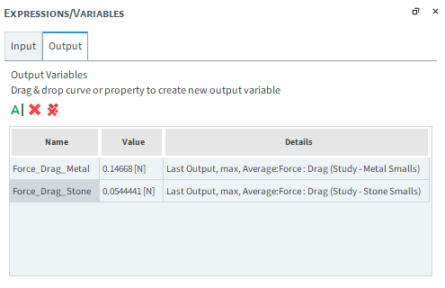
Tip: Your values may differ from the ones presented in this tutorial.
You can also color your Metal Smalls and Stone Smalls by Drag Force (as shown).
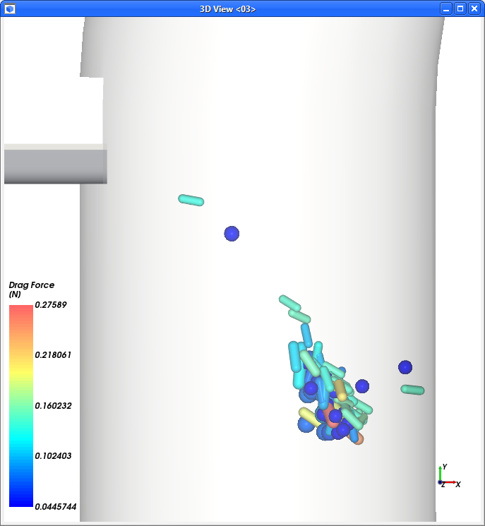
Use the information in the table below to check your results.
Step Data Entity Editors Location Parameter or Action Settings A User Processes ﹂Metal Smalls
Coloring Nodes (Enabled) Nodes | Property Drag Force ⯆ B ... ﹂Stone Smalls
Nodes (Enabled) Nodes | Property Drag Force ⯆
Note that the drag forces calculation depends on the particle shape, orientation, size, velocity and other properties.
Also note that we are visualizing a Particles Time Selection, which shows the particles we've chosen to filter at the position they were just before they left the region specified, for all times in the simulation. The visualization does not change with time because the selection itself includes multiple times.
Another way to evaluate these results is to take a closer look at the two outlets to analyze what kind of particles are passing through each end of the pipe.
We will do this by creating two Cube User Processes:
One for the outlet (at the top)
Another for the inlet (at the bottom)
We will then use again Particle Time Selection to evaluate which Particle Groups go through each Cube.
Use the information in the table that follows to create these User Processes.
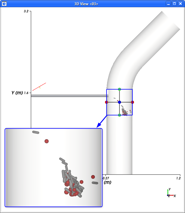
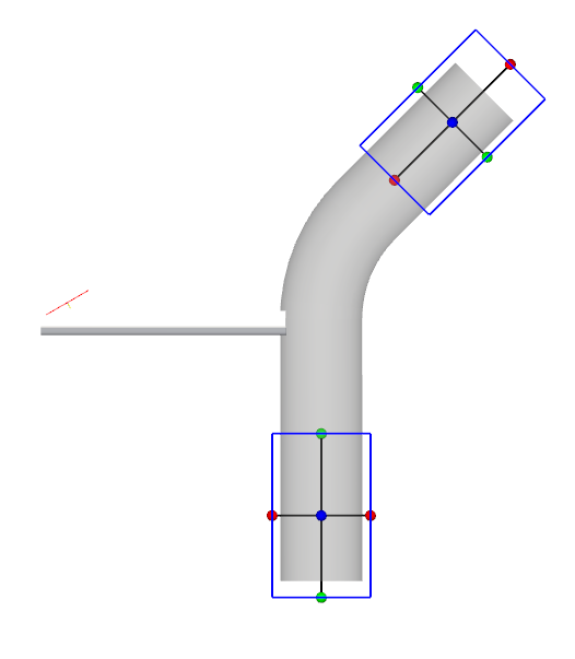
Step Data Entity Editors Location Parameter or Action Settings A Particles Create a Cube User Process B User Processes ﹂Cube <03>
Cube Name Outlet Center 0.7, 2.7, 0 [m] Magnitude 1, 0.6, 0.6 [m] Cube | Orientation Method Angles ⯆ Rotation 0, 0, 45 [dega] C Particles Create a Cube User Process D User Processes ﹂Cube <03>
Cube Name Inlet Center 0, 0.4, 0 [m] Magnitude 0.6, 1, 0.6 [m]
The placements of the two Cubes are shown below.
Using these two Cubes, we can now create a Particle Time Selection to evaluate which particles are passing through each outlet.
Use the table below to create the Particles Time Selection User Processes.
Step Data Entity Editors Location Parameter or Action Settings A User Processes ﹂Outlet
Create a Particles Time Selection User Process B User Processes ﹂Particles Time Selection <02>
Time Selection Name Outlet All Time Domain Range All ⯆ C User Processes ﹂Inlet
Create a Particles Time Selection User Process D User Processes ﹂Particles Time Selection
Time Selection Name Inlet All Time Domain Range All ⯆ Now that we have our user processes, let's plot them.
Use the information in the table that follows to define a histogram.
Step Item Parameter or Action Settings A User Processes ﹂Outlet All Time
Show in new Histogram by Particle Group B Histogram (window) Configure Histogram (button) C Configure Histogram (dialog box) Weigth Particle Mass ⯆ Number of Bins 4 [ - ] Percent Values (Enabled) Properties Particle Group Limits User Defined ⯆ Min 0 [<ind>] Max 4 [<ind>] D User Processes ﹂Inlet All Time
Show in current Histogram by Particle Group
Results of the Histogram are shown. Take note the following:
The 1st and 3rd bins are Metal and Stone particles, respectively. Only the (lower) Inlet (in orange) had these groups.
The 2nd and 4th bins are Paper and Wood particles, respectively. Only the (upper) Outlet (in black) had these groups.
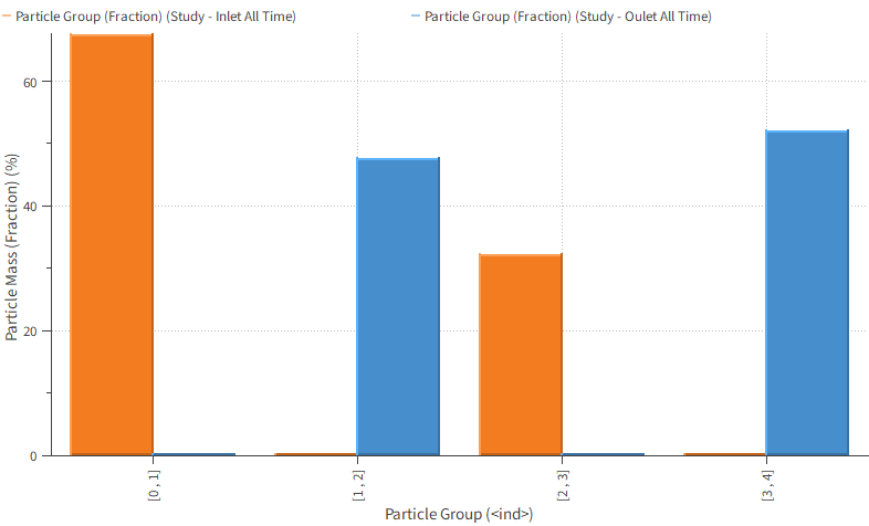
Using these results, we can conclude that:
The lighter and flatter Paper and Wood particles were more affected by the drag force than by the gravity force, and were therefore carried up the pipe.
The heavier and thicker Metal and Stone particles were more affected by the gravity force than by the drag force, and therefore fell down the pipe.
This completes Part C of this tutorial, in which Ansys Workbench was used to set up, run, and post-process a one-way coupled simulation between Rocky and Ansys Fluent.
During this tutorial, it was possible to:
Apply Fluent CFD results to the Rocky project through Workbench.
Set up the fluid forces models in Rocky.
View a slice of the fluid vectors in Rocky.
Process the one-way coupled simulation in Rocky.
Analyze particle flow, temperature, and drag effects.
What's Next? If you completed this tutorial successfully, then you are ready to move on to next tutorial.