


- Fringe Component
Display fringe component data on the model.
- Fringe Range
Set fringe and Iso-surface ranges.
- History
Display and plot data for various data over time.
- XyPlot
Control all open XY-Plot windows and files using this interface.
- ASCII
Browse and display data in LS_DYNA ASCII output files.
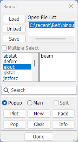
- BinOut
Browse, display, and compare data stored in binary output files.
- Follow
Set a reference point/plane for animations.
- Trace
Trace the paths of nodes over time.
- State
Activate/deactivate time states and apply overlays to the model.
- Particle
Particle method interface.
- Chain Model
Chain multiple models together for animation.
- Fld
Interface for metal forming analysis.
- Output
Output model data.
- Setting
Organize personal display preferences.
- Vector
Display normal vectors for any element in the model.
The FComp interface is used to display fringe component data on the model. It allows the selection of various scalar quantities like strains and stresses that can be fringed.
For shells and beams, such data is stored for different integration points through their thicknesses and cross sections respectively. Upon selecting a component to be fringed, further selection of data at a particular integration point can be made using a simple selection widget with options (Low/Mid/Upp/Max/Ave/Min/IPt/BPt).
By default LS-PrePost will fringe the maximum of all integration point data available.
Stresses and strains in d3plot are in the global coordinate system except when CMPFLG have been used. By default, LS-PrePost will plot the stress and strain as they are written to d3plot. The stress and strain can be plotted in Element, Global, Material or in a User specified coordinate system by changing the "d3plot/Elem/Glob/Mtrl/User" switch but this requires that both the d3plot and the keyword file have been read.
Load data using the button and fringed. This can be from external third party software or element and nodal results output from the Output Interface in Post.
- Basic
General functions for displaying fringe components.
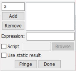
- Fringe expression
Display fringe components with formular expression.
Sample
- Sample
A sample show how to use basic functions to fringe the model.
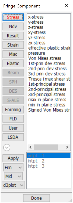
- Fringe Component List
Fringe Component selection menu.
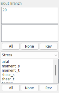
- Stress
Global Stress/Strain components.
- Ndv
Nodal Displacement/Velocity Contour.
- Result
Stress resultant components.
- Strain
Logarithmic strain components.
- Misc
Pressure, Temperature, Thickness, etc.
- Elastic
Elastic strains.
- Beam
Beam fringe components.
- SPH
Special SPH fringe components.
- DES
Special DES fringe components.
- S-ALE
S-ALE, Dynaauto, ISPG fringe components.
- Forming
Forming components.
- FLD
FLD strain components.
- User
User defined fringe components.
- LSDA
Lsda defined fringe components.
- Apply
Collect fringe data.
- Frin Choice
Choose fringe method (Frin/Isos/Lcon/Fiso/XFrn/FMes).
- Max Choice
Set shell stress surface position and integration points (Low/Mid/Upp/Max/Ave/Min/IPt/BPt).
- Coordinate System Choice
Plot stress and strain as they are in d3plot or in: Element, Global, Material or a User specified coordinate system. The "User" specified system is specified (per part) in Settings - General Settings - Local Coord System.
- Integration Point List
Select shell integration point.
- Variable name text
Enter a variable name (max 8-char).
- Add
Move component from fcomp interface to list.
- Remove
Remove selected component from list.
- Component definition list
List the definition of components.
- Expression
Enter formular expression in the text widget.
- Single Time Step
Only apply fringe expression to one state.
- Fringe
Fringe data according to expression.
- Done
Exit fcomp expression interface.
Use this interface to set fringe and Iso-surface ranges.
- Basic
General functions for setting fringe range.
- Fringe color palette
Set fringe color palette.
Sample
- Sample
A sample to show how to set Limit fringe color map to lower and upper user range.
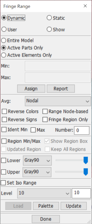
- Dynamic
A set of min/max ranges is computed for each time state.
- Static
A constant min/max range is computed using all time states.
- User
Range set by user, enter min/max values below.
- Show
Show elements within the range entered below.
- Entire Model
Range computed for entire model.
- Active Parts Only
Range computed for active parts only.
- Active Elements Only
Range computed for active elements only.
- Min
Assign current range to user min.
- Max
Assign current range to user max.
- Assign
Assign current range to user min/max.
- Report
Report the element number distribution.
- Avg
Element to node averaging scheme.
- Reverse Colors
Reverse the fringe color palette.
- Range Node-based
Update the fringe max and min based on the nodal scalar.
- Reverse Signs
Reverse the interforce file pressure sign.
- Fringe Region Only
Set gray fringe outside the defined region.
- Ident Min
Identify first N minimum values.
- Max
Identify first N maximum values.
- Number
Enter number of min/max values to be identified (N).
- Region Min/Max
Show min and max values for region - use Zin to define.
- Show Region Box
Show the region box.
- Updated Region
Change the Min and Max region as model gets zoomed or panned.
- Keep All Regions
Keep all identified region info on graphics area.
- Lower
Set Limit fringe color map to lower user range. Select color for lower user range fringe. Change the lower fringe transparence.
- Upper
Set Limit fringe color map to upper user range. Select color for upper user range fringe. Change the upper fringe transparency.
- Set Iso Range
Set Isosurface range values independently.
- Level
Set and enter number of colors in fringe palette.
- Load
Load Fringe partition value and color for Legend,Each line in the file should contain 4 values:
Legend_value R G B
Where R G B are the color components in range 0.0 to 1.0.
- Palette
Open fringe color palette. See below in details.
- Update
Update range settings.
- Done
Exit Fringe Range interface.
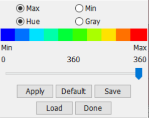
- Max
Set fringe color for maximum of range.
- Min
Set fringe color for minimum of range.
- Hue
Use slider bar to set Hue color value.
- Gray
Use slider bar to set Gray shade value.
- Apply
Apply current palette to the fringe plot.
- Default
Reset fringe palette to default values.
- Save
Save fringe color palette to a file.
- Load
Load fringe color palette from a file.
- Done
Exit fringe palette interface.
This interface is used to display and plot data for various data over time. It allows selection of various nodal, element, and material quantities from binary files like d3plot, d3dtht etc...
Depending on the type of binary files loaded, the list of available components will change. Time history plotting data from d3plot files is also possible. However, typically a d3plot file contains data for state animation. Consequently the resolution of time history is limited to the number of states in d3plot files. For higher resolution time history plotting, either d3thdt, binout, or various ASCII files should be used.
- Basic
Basic functions to display various components.
- Affixation
Affixation functions, such as volume fail options.
Sample
- Sample
A sample to show how to plot element component history value.
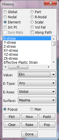
- Global
Select global history plot.
- Nodal
Select nodal history plot.
- Element
Select element history plot.
- Int Pt
Select element integration point history plot.
- Part
Select material history plot.
- R-Nodal
Select relative nodal history plot.
- Scalar
Select fringed scalar history plot.
- Vol Fail
Select volume of material failure option.
- Sum Mats
Sum materials for material history plot.
- Along Path
Plot fringe value along selected path.
- Component list
Select a time history component.
- Value
Select element values or max/min element value for material.
- E-Type
Select element type for time history plotting.
- E-Axes
Select shell element axes for time history plotting.
- Surface
Select shell stress surface position.
- Popup
Show XY-Data in Popup window.
- Main
Show XY-Data in Main Window.
- Plot
Plot time history data in current XY-plot window.
- New
Plot time history data in a new XY-plot window.
- Padd
Add time history data to current XY-plot window.
- Clear
Clear picked entities.
- Raise
Raise all open XY-plot windows or current page.
- Pop
Open and Raise all closed XY-plot windows or current page.
- Done
Exit Time History Results interface.
Volume fail options:
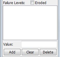
- Eroded
Add item to failure list.
- Failure Levels List
Select failure levels from list.
- Value
Enter failure level value to be added to the list.
- Add
Add entered value to the failure levels list.
- Clear
Clear text field and selected items.
- Delete
Delete selected item from the failure levels list.
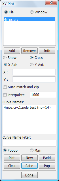
This interface is used to control all open XY-Plot windows and files. External XY data can be loaded for plotting and/or cross plotting.
Often there is need to plot force vs. deflection response of structures. This requires a force vs. time curve and a deflection vs. time curve. Cross plotting allows users to select deflection from the deflection vs. time curve for the x-axis and force from the force vs. time curve for the y-axis. If the number of points for the 2 curves is not the same, the data is interpolated.
Cross plotting can also be done from plot read in by using the Add button or from XY-plot windows. For cross plotting data from XY-plot windows, the Window option should be activated (The default is the File option).
The format of external XY data can be in Microsoft CSV format or XY data pairs as shown below. In this example, note how the first line of each curve definition defines the number of XY data pairs that follow:
2
0.0,0.0
10.0,20.0
4
0.0,0.0
30.0,20.0
40.0,10.0
50,0,10.0
- Show
Show selected plots.
- Cross
Cross selected plots.
Sample
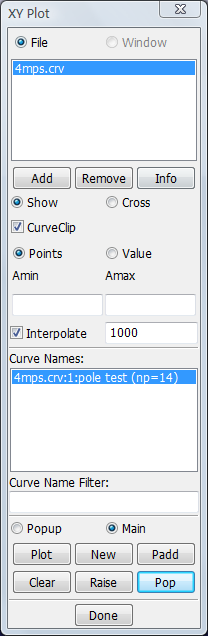
- File
Show list of XY-Plot data files.
- Window
Show list of current XY-Plot windows.
- File/Window list
Select file/window to be shown.
- Add
Open and add a XY-Plot data file to the filename list.
- Remove
Remove a XY-Plot data file from the filename list.
- Info
Show full XY-Plot data file path in command window.
- Show
Show selected plot.
- Cross
Cross selected plots.
- CurveClip
Clip curves before plotting.
- Points
Enter start and end clip points.
- Value
Enter start and end clip values.
- Amin
Enter minimum abscissa point or value.
- Amax
Enter maximum abscissa point or value.
- Interpolate
Linearly interpolate curves before plotting.
- Curve Names List
Select curve to show or to crossplot.
- Curve Name Filter
Enter text for name filter, clear to reset (must press enter).
- Popup
Show XY-Data in Popup window.
- Main
Show XY-Data in Main Window.
- Plot
Plot XY-Plot data in current XY-Plot window.
- New
Plot XY-Plot data in a new XY-Plot window.
- Padd
Add XY-Plot data to current XY-Plot window.
- Clear
Clear selected items in list.
- Raise
Raise all open XY-Plot windows or current page.
- Pop
Open and Raise all closed XY-Plot windows or current page.
- Done
Exit Cross Plotting interface.
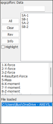
This interface is used to browse and plot time history data contained in various ASCII databases written by LS_DYNA like nodout, secforc etc...
There are approximately 30 different files that can be processed through this interface. Similar time history data output by LS_DYNA and beyond in binary files called binout can be processed using the Binout Interface.
- Basic
Basic functions for every ascii file.
- Affixation
Added functions for some ascii especial files, such as spcforc, jntforc etc.
Sample
- Sample
A sample to show how to use it.
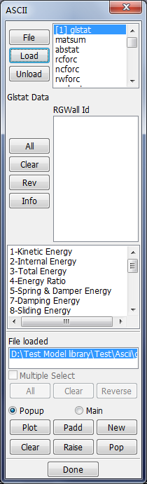
- Ascii type list
Select ascii file type.
- File
Load an ASCII file from an alternative directory.
- Load
Load existing file for selected ASCII file type.
- Unload
Un-Load selected ASCII file (to free memory).
- Id selection list
Select the Id to show.
- All
Select all ASCII items.
- Clear
Clear all selections.
- Rev
Reverse selection.
- Info
Show information on the loaded ASCII file.
- Component Selection list
Select compnoent to show.
- File loaded list
Select an ascii file or multipe ascii files for processing.
- Multiple Select
Set single or multiple selection on list.
- All
Select all loaded files.
- Clear
Clear all selection.
- Reverse
Reverse selection.
- Popup
Show XY-Data in Popup window.
- Main
Show XY-Data in Main Window.
- Plot
Plot items from ASCII file in current XY-plot window.
- Padd
Add items from ASCII file to current XY-plot window.
- New
Plot items from ASCII file in a new XY-plot window.
- Clear
Clear picked entities.
- Raise
Raise all open XY-plot windows or current page.
- Pop
Open and Raise all closed XY-plot windows or current page.
- Done
Exit ASCII File Operation interface.
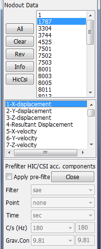
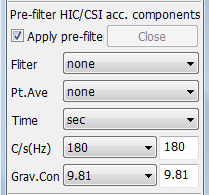
- HicCsi
Open Hic/Csi pre-filter options interface.
- Apply pre-filter
Apply filtering on acc. components prior to calculate HIC/CSI .
- Filter
Select filter to apply.
- Point
Select number of points to average.
- Time
Select time unit for filtering and hic/csi calculation.
- C/s (Hz)
Select and enter frequency.
- Grav.Con
Select and enter gravity constant.
- Done
Close HIC/CSI pre-filter panel.
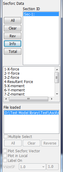
- Total
Toggle the combining of multiple ASCII items.
- Plot Secforc Vector
Plot Secforc vectors for selected sections.
- Plot in Local
Plot Secforc vectors in local plane system.
- Label On
Turn on label of the section force vectors.
- VsizeSF
Select and enter scale factor for vector size.
This interface facilitates the plotting of time history data from binary database output generated by LS_DYNA versions ls970 and newer. The contents of these binary files is the same as ASCII files except these files are stored as branches in a single binary file from smp versions of LS_DYNA. The branch system makes it easy to navigate and there is even the option to open multiple files for comparison. Note that the mpp version of ls970 produces a series of binout files: binout0000, binout0001, etc...
- Basic
Basic functions for reading BINOUT file.
- Affixation
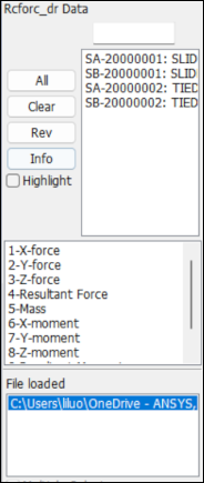
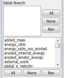
Added functions for sub branches, such as Abstat_cpm, Deforc, Elout, Glstat, Matsum, Nodfor, Rbdout, Rcforc, Sleout, Spcforc, Swforc, Output, HIC/CSI and so on.
Sample
- Sample
A sample to show how to use binary database output.
- Plot
Plot selected component in current XY-Plot window.
- New
Plot selected component in a new XY-Plot window.
- Padd
Add selected component to current XY-Plot window.
- Pop
Open and Raise all closed XY-Plot windows or current page.
- Clear
Clear list selections.
- Info
Show the general information about the current selections.
- Sub branch list
Sub-branches for the BINOUT file.
- Popup
Show XY-Data in Popup window.
- Main
Show XY-Data in Main Window.
- Load
Load a BINOUT file.
- Unload
Un-load a BINOUT file.
- Save
Save a BINOUT branch to a file.
- Search
Search and select branch items. Separate multiple search strings with commas. FromID: ToID selects a range of IDs. Free text searching with
*and?is allowed. The option "-id" searches the first token on each item. The option "-heading" searches all except the first token.- Open file list
BINOUT files currently opened.
- Main branch list
Main branches in the BINOUT file.
- Done
Exit BINOUT interface.
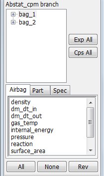
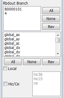
- Abstat_cpm branch list
Select entities for the Abstat_cpm branch.
- Exp All
Expand all entities.
- Cps All
Collapse the tree.
- Airbag
Select gas particle components for the airbag entities.
- Part
Select gas particle components for the part entities.
- Spec
Select gas particle components for the spec entities.
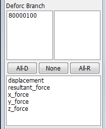
- Left list
Select Deforc displacement entities.
- Right list
Select Deforc torsional enitites.
- All-D
Select all displacement entities.
- None
De-select all entities.
- All-R
Select all torsional entities.
- Component list
Select Deforc component.
- Element id list
Select element ids (and nip).
- Integration points list
Select integration points with element ids.
- All
Add all possible combinations of element ids and integration points.
- None
Remove all item from element list.
- Revert
Reverse the previous action.
- Stress, Strain, Muscle, or History Choice
Choose an available component: stress, strain, muscle, or history.
- Component list
Select components to plot.
- All
Select all components.
- None
De-select all components.
- Rev
Reverse the previous selection.
- Entity list
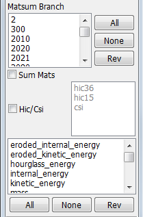
Select materials for matsum plot.
- Sum Mats
Sum component result through all selected materials.
- Hic/Csi
Turn on/off the Hic/Csi panel.
- Hic/Csi list
Select head injury criteria / chest injury options.
- Component list
Select components to plot.
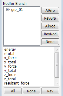
- Entity list
Select entities for output.
- AllGrp
Select all entities in group form.
- RevGrp
Reverse selections in group form.
- AllNod
Select all entities in nodal form.
- RevNod
Reverse selections in nodal form.
- None
De-select all entities.
- Component list
Select components to plot.
- Entity list
Select the entities.
- All
Select all entities.
- None
De-select all entities.
- Rev
Reverse the previous selection.
- Component list
Select the components.
- All
Select all components.
- None
De-select all components.
- Rev
Reverse the previous selection.
- Local
Switch to local components.
- Hic/Csi
Turn on/off the Hic/Csi panel.
- Hic/Csi list
Head injury criteria / chest injury options.
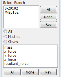
- All Radion button
List both slave and master sides of the contacts.
- Masters
List only master sides of the contacts.
- Slaves
List only slave sides of the contacts.
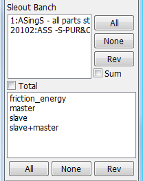
- Sum
Sum over the selected entity with selected componets.
- Total
Toggle total components.
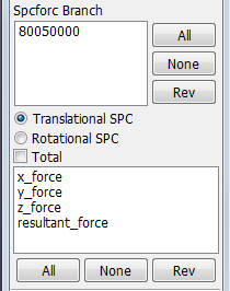
- Translational SPC
List only SPC nodes that has translational forces.
- Rotational SPC
List only SPC nodes that has rotational moments.
- Total
Sum the result for all selected entites.
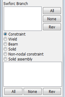
- Constraint
List only constraint spot weld type.
- Weld
List only weld spot weld type.
- Beam
List only beam spot weld type.
- Solid
List only solid spot weld type.
- Non-nodal constraint
List only non-nodal spot weld type.
- Solid assembly
List only solid assembly spot weld type.
- Write out branches list
Select to remove the branch from write-out list.
- All
Write out all branches.
- None
Clean up current selected branches.
- Rev
Select the branches not currently selected.
- As ASCII(es)
Export selected binout branches as ascii databases.
- File name
Enter a file to write out the selected branches and browse the directory.
- Apply
Write out selected branches to a file.
- Done
Exit save interface.
- Apply pre-filter
Apply filtering on acc. components prior to calculate HIC/CSI.
- Fliter
Select filter to apply.
- Pt.Ave
Select number of points to average.
- Time
Select time unit for filtering and hic/csi calculation.
- C/s(Hz)
Select and enter frequence.
- Grav.Con
Select and enter gravity constant.
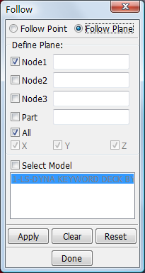
The Follow interface is generally used in conjunction with model animation. Choose either a single point or a plane which will then be frozen and displayed in the center of the screen at all times during the animation.
If the structure is undergoing large rigid body translation or rotation as it is crushing, often it is difficult to understand how the structure is deforming relative to some point in the structure. The Follow Point option allows freezing of the displacement of a follow point (node picked to freeze). Follow Plane is for removing rotations of a body undergoing large rotations, such as tires, a brake rotor, or even an entire vehicle.
Follow plane has an additional option to select parts to freeze rotation as opposed to the whole model (all parts). Follow settings are retained upon exiting this interface and entering another interface. The Reset button disables the follow point and follow plane.
- Follow Point
Choose single node to follow.
- Follow Plane
Choose plane to follow.
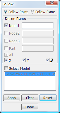
- Node1
Enter ID for Node 1.(Follow point mode can select only 1 node.)
- X/Y/Z
Select X/Y/Z direction to follow.
- Select Model
Select Model When multiple models are loaded, this opens a menu in region Model List from which to choose the model that Follow will apply to.
- Model List
Display all models.
- Apply
Apply follow to model view.
- Clear
Clear pick list.
- Reset
Deactivate follow mode and restore model to previous position.
- Done
Exit Follow interface.
This interface is used to trace the paths of nodes over time (note that it is available for post-processing only). The trajectory of nodes can be displayed by selecting them using the General Selection Interface and then playing the animation using the Animation Controls (which can be accessed by clicking the Anim Rendering Button). The plotted traces can be output in several forms (displacement curves, coordinate histories, or *BOUNDARY_PRESCRIBED_MOTION_NODE). This data is often used to define prescribed motion for sub-system models.
- Node Trace
Selected Node Trace menu.
- Streamline
Selected Streamline menu.
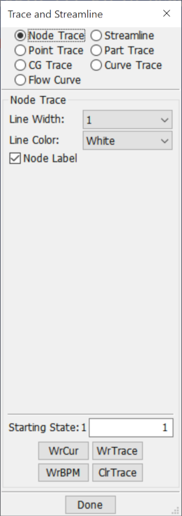
- Line Width
Select trace line width.
- Line Color
Select trace line color.
- Node Label
Turn node label on/off.
- Staring State
Enter starting state number.
- WrCur
Write displacements as *DEFINE_CURVEs for selected nodes.
- WrTrace
Write coordinate history of selected nodes.
- WrBPM
Write trace node motion as *BOUNDARY_PRESCRIBED_MOTION_NODE.
- ClrTrace
Clear traced entities.
- Done
Exit Node Trace interface.
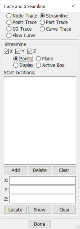
- Vector Type
Select vector type. This will be shown only you load a mutiple solver model.
- X/Y/Z component of vector
Select X/Y/Z componet of vector.
- Add
Add current point to point list.
- Delete
Delete selected point from list.
- Clear
Delete all points from list.
- X/Y/Z
Current X/Y/Z coordinate picked or entered.
- Locate
Find and plot start points on model.
- Show
Caculate and show streamlines on model.
- Clear
Remove streamlines from model.
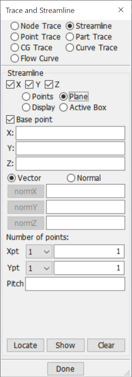
- Base point
Pick base point for plane.
- X/Y/Z
Base X/Y/Z coordinate picked or entered.
- Vector
Pick head of vector from base point.
- Normal
Pick direction of plane normal from base point.
- normX/normY/normZ
normX/normY/normZ direction.
- Xpt/Ypt
Number of point in X/Y direction.
- Pitch
Distance between points in plane.
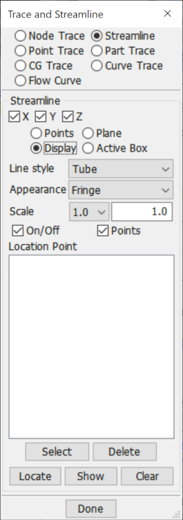
- Line style
Select streamline display type.
- Appearance
Select streamline appearance.
- Scale Option
Scale relative width for streamlines.
- Scale Text Feild
Enter scale relative width for streamlines.
- On/Off check box
Switch streamline display on or off.
- Points check box
Switch streamline start point on or off.
- Location Point
List of separately defined planes of location points.
- Select
Show only selected defined planes of streamlines.
- Delete
Delete selected defined planes of streamlines.
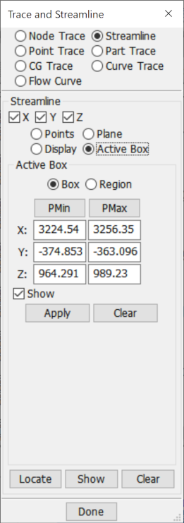
- Box
Use entity seletion get box max and min value.
- Region
Use genseletion get region max and min value.
- PMin/PMax
Call Position Dialog to get position.
- X/Y/Z
Enter X/Y/Z coordinates of the minimum/maximum point.
- Show
Show outline of active box.
- Apply
Set active box.
- Clear
clear/delete active box.
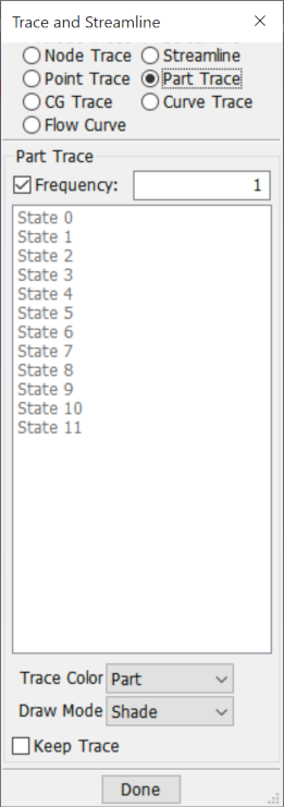
- Frequency
Set part trace frequency.
- Trace Color
Select trace part color.
- Draw Mode
Select part trace draw mode.
- Line Width
Select trace line width.
- Line Color
Select trace line color.
- Part CG
Change to trace part cg for every selected part.
- No Line
Change to not draw the lines.
- Starting State
Enter starting state no.
- ClrTrace
Clear traced entities.
- Show
Show the trace of cg for selected elements or parts.
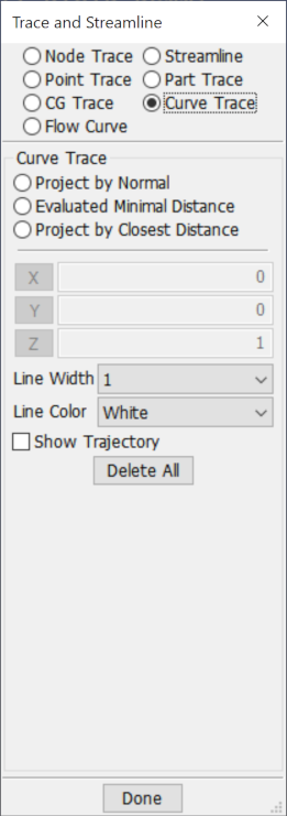
- project by normal
Project by ray intersection with mesh.
- Evaluated Minimal Distance
Searching a point with evaluated minimal distance onto mesh.
- Project by Closest Distance
Searching a point with minimal distance onto mesh.
- X/Y/Z button
Set normal as (1, 0, 0) / (0, 1, 0) / (0,0,1).
- X/Y/Z text control
Enter head of vector x/y/z component.
- Line Width
Select trace line width.
- Line Color
Select trace line color.
- Delete All
Delete all curve tracing.
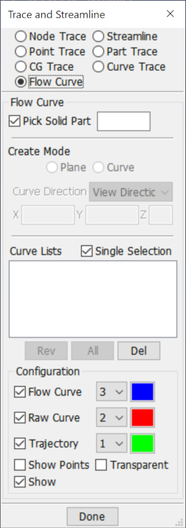
- Pick Solid Part
Pick solid part which curve flows inside.
- Plane
Using a plane to cut solid, and generate curves cluster in the cutting plane.
- Curve
Insert a curve into the solid inside.
- Curve Direction
Curve's direction.
- Single Selection
Only one plane or curve visible in the view.
- Rev
Reverse selection (hide/show).
- All
Select all flow curves and show all.
- Del
Delete all the selected(shown) curves.
- Flow Curve
Show or hide current flow curve,Set flow curve width and color.
- Raw Curve
Show or hide raw curve,Set raw curve width and color.
- Trajectory
Show or hide current flow curve,Set trajectory width and color.
- Show Points
Show all points from curve.
- Transparent
Draw transparent.
- Show
Show or hide result after dialog close.
Use this interface to activate/deactivate time states and apply overlays to the model.
- Select
Display selected state.
- Inactive
Make selected inactive.
- Delete
Delete selected state permanently.
- MultiState
Display multiple states on graphics window.
Sample
- Sample
The samples to show how to use it.
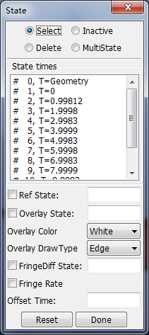
- State times
State list.
- Ref State
Change displacement referent state on/off. Enter reference state for displacements.
- Overlay State
Turn overlay mode on/off. Enter state numer for overlay or inactive.
- Overlay Color
Select overlay color.
- Overlay Draw Type
Select overlay type.
- Fringe Diff State
Set to difference fringe mode. Enter state number for difference fringe.
- Fringe Rate
Set fringe to rate of changing mode.
The same as Select
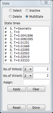
- No. of WHoriz
Select and enter number of windows in horizontal direction .
- No. of WVerti
Select and enter number of windows in vertival direction .
- Assign
Enter states numbers for all subwindows. (For example - 1st:last:inc)
- Apply
Apply multiple states rendering.
- Clear
Clear multiple states rendering.
- Reset
Reset all states to active.
- Done
Exit state time/overlay interface.
The particle interface is used to simulate the gas generated to inflate airbags. The particles maybe have mass and momentum and act on the surfaces of the bag to expand it. A model can have several bags and the bags surface has porosity and vent holes for the gas to escape. Showing the particles and there movement helps to illustrate how the gas moves into and around the bag as it inflates. When a model including particles is loaded, the particle interface will be shown, or this interface can't be shown.
- Basic
Operations of showing particles and changing particles' color and type in bags and gas mixtures.
- Plot Velocity Distribution
Show the area of plotting velocity distribution function.
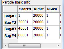
- Particle Basic Info
Show bags information for the particle model.
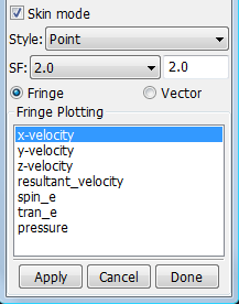
- Fringe
Show fringe plotting.
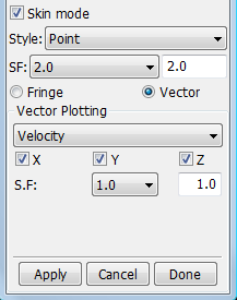
- Vector
Show vector plotting.
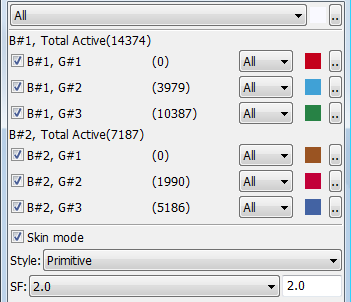
- Top menu
Show particles in all bags and all gas mixtures.
- Top color button
Change color for selected particle type.
- B#NO.G#NO. check box
Show particles for bag#NO.gas#NO.
- B#NO.G#NO. menu
Choose a different displaying particle type.
- B#NO.G#NO. color button
Choose a differnet color for the gas component.
- Skin mode
Toggle between skin and interior mode.
- Style
Select particle display style.
- SF
Choose and enter a scale factor for particle size.
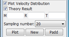
- Plot Velocity Distribution
Show the area of plotting velocity distribution function.
- Theory Result
Show the velocity distribution theory results.
- M
Molar mass.
- R
Universal Gas Constant.
- T
Temperature.
- Sampling number
Select sampling number when plotting the velocity distribution.
- Plot
Plot velocity distribution curve in current xy-window.
- New
Plot velocity distribution curve in new xy-window.
- Padd
Add velocity distribution curve in current xy-window.
- Fringe
Show fringe plotting.
- Vector
Show vector plotting.
- Fringe components list
Select an available component to fringe.
- Apply
Apply fringe.
- Cancel
Remove fringe.
Multi-step analyses are often conducted in separate phases as individual LS_DYNA runs. For each run a set of binary d3plot files is produced, and each set of plots starts time of T=0.0.
This interface allows chaining individual sets of d3plot files into a single animation sequence
Sample
- Sample
A sample to show how to use it.
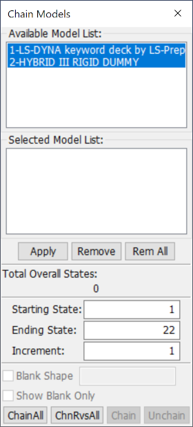
- Available Model List
List of currently loaded d3plot sets.
- Selected Model List
List of plot sets that will be chained.
- Apply
Apply chaining to this model.
- Remove
Remove this model from chaining.
- Rem All
Remove all models from chaining.
- Starting State
Enter the starting state number.
- Ending State
Enter the ending state number.
- Increment
Enter the state increment number.
- Blank Shape
Show the final shape of blank.
- Show Blank Only
Show Blank Only.
- ChainAll
Apply chaining to all models.
- ChnRvsAll
Apply chaining to all models in the opposite order.
- Chain
Apply chaining to all selected models.
- Unchain
Unchain selected models.
This interface is used for metal forming analyses. An example of the correct format to use when loading an external FLD data file is shown below. The second line ("8" in the example) should be set equal to the number of coordinate pairs that follow (one pair per line).
- Plot
Plot FLD diagram in current XY-Plot window.
- New
Plot FLD diagram data in a new XY-Plot window.
- Padd
Add data to FLD diagram in current XY-Plot window.
- Clear
Clear picked entities.
- Raise
Raise all open XY-Plot windows.
- Pop
Open and Raise all closed XY-Plot window.
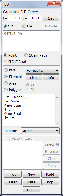
- t
Enter sheet thickness in mm.
- n
Enter fld crit. formula index.
- Set
Apply the new t and n values.
- t_n
Set thickness and index of FLD curve.
- File
Read thickness and index of FLD curve from a file.
- Browse
Open flc data file.
- Point
Select an item for point on FLD plot.
- Strain Path
Select an item for tracer on FLD plot.
- FLD E'Strain
Toggle FLD Strain (Engineering/True).
- Part
Select a material for FLD plot.
- Element
Select an element for FLD plot.
- Area
Define an area for FLD plot.
- Polygon
Define a region for FLD plot.
- Clear
Clear information in popup windows.
- Info
Open/Close FLD information dialog.
- In
Select entities within the area/polygon.
- Out
Select entities outside the area/polygon.
- Position
Select shell surface for FLD results.
This interface is used to output model data. During post-processing of binary d3plot files, often there is a need to write entire or partial models out at a particular state in various third party formats as well as in LS_DYNA keyword file format. Such output is often used for conducting analysis like spring-back followed by crash analysis.
In additions to this, the output can be limited to only nodal coordinates, element definitions, nodal velocities, element results, nodal results, shell principal strains, shell element thicknesses, and fluid surfaces. Fluid surfaces are only available if fluid data is present from ALE simulations in d3plot files. Output of a number of states can be saved to a single file by activating the Append option.
- Basic
Basic functions to write model data to files.
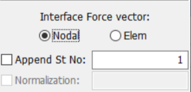
- Affixation
Added options for interface force file. When the file loaded is interface force file, this area will be shown.
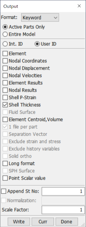
- Format
Select output format.
- Active Parts Only
Write data for the active parts and elements only.
- Entire Model
Write data for the entire model.
- Int.ID
Write elements and nodes using internal ID.
- User ID
Write elements and nodes using user ID.
- Element
Write element connectivities to file.
- Nodal Coordinates
Write nodal coordinates to file.
- Nodal Displacment
Write nodal displacements to file.
- Nodal Velocities
Write nodal velocities to file.
- Element Results
Write element results to file.
- Nodal Results
Write nodal results to file.
- Shell P-Strain
Write shell principal strain to file.
- Shell Thickness
Write shell element thickness to file.
- Fluid Surface
Write fluid surface segments to file.
- Element Centroid
Write element centroid coordinates to file.
- 1 file per part
Write each part to a different file.
- Separation Vector
Write part separation vectors to file.
- Exclude strain and stress
Don't output shell thickness, initial stress and strain. Only available when output dynain ASCII file.
- Exclude history variables
Don't output history variables.
- Solid ortho
Elements using orthotropic material are written as *ELEMENT_SOLID_ORTHO, with directions corresponding to the material directions. Only available when output dynain ASCII file.
- Long format
Output keyword on long format.
- SPH Surface
Write SPH surface segments to file.
- Point Scalar value
Write point scalar value.
- Append
Select to append data to an existing file.
- St No
Enter state sequence to be written (eg 1:5:2).
- Normalization
A factor that is inside d3eigv for normalization of the eigenvector.
- Scale Factor
Scale factor for nodal coordinates and displacements. Only active when output Keyword format.
- Write
Start writing to file.
- Curr
Write data for current state.
- Done
Exit File Writing interface.
This interface is used to organize general personal display preferences. You can set various quantities for the entire model or for parts.
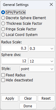
- SPH/Particle
Open SPH/Particle display options interface.
- Discrete Sphere Element
Open Discrete sphere element display options interface.
- Thickness Scale Factor
Open shell thickness scale factor interface.
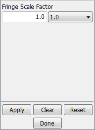
- Fringe Scale Factor
Open fringe scale factor interface.
- Local Coord System
Open local coordinate system interface.
- Apply
Apply selected options to model.
- Clear
Clear any picked parts from list.
- Reset
Reset model to default options.
This function could set factor to change display of SPH mode. See sample.
- Radius Scale
Select SPH radius scale factor.
- Sphere divs
Select SPH sphere divisions.
- Style
Select SPH sphere style.
- Fixed Radius
Keep SPH radius constant.
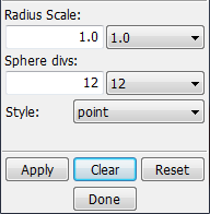
- Radius Scale
Enter radius scale factor.
- Sphere divs
Enter sphere divisions.
- Style
Select SPH sphere style.
This function is to change thickness scale factor. Use the Appearance interface and check Thickfirst.
- Whole/Part
Apply to whole/part model.
- Thickness Scale Factor
Select thickness scale factor.
- Change in Thickness Scale
Select thickness scale factor.
- Shell Thickness
Enter shell inital thickness for % reduction fringe.
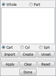
- Whole/Part
Apply to whole/part model.
- Cart
Local system is cartesian system.
- Cyl
Local system is cylindrical system.
- Sph
Local system is spherical system.
- Import
Click to import coordinate system from keyword file.
- Create
Click to create new coordinate system.
- Unset
Click to unset the active coordinate system.
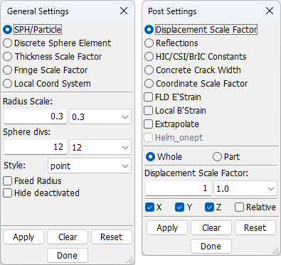
This interface is used to organize personal post-processing display preferences. You can set various quantities for the entire model or by parts.
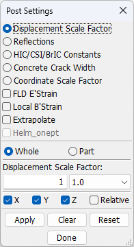
- Displacement Scale Factor
Open displacement scale factor interface.
- Reflections
Open global reflections interface.
- HIC/CSI/BrIC Constants
Open Head Injury Criteria/Chest Severity Index constants interface.
- Concrete Crack Width
Open concrete crack width interface.
- Coordinate Scale Factor
- FLD E'Strain
Toggle FLD Engineering/True Strain.
- Local B'Strain
Toggle Local Brick Strain (For solid element strains rotated to assumed local axes - not recommended for normal use).
- Apply
Apply selected options to the model.
- Clear
Clear and picked parts from the list.
- Reset
Reset model to default options.
Sample
See each interface introduction .
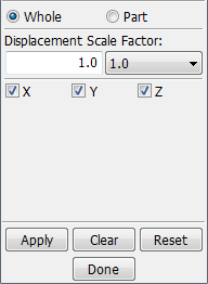
- Whole/Part
Apply to whole/part model.
- Displacement Scale Factor
Select displacement scale factor.
- X/Y/Z
Displacement model in X/Y/Z direction.
This function is to reflect model about a plane. See sample.
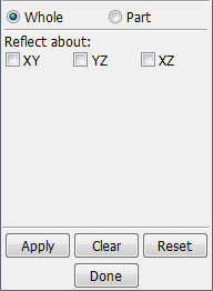
- Whole/Part
Apply to whole model. Select the whole model to reflection.
- XY
Reflect model about XY plane.
- YZ
Reflect model about YZ plane.
- XZ
Reflect model about XZ plane.
Time and Gravity constants for Head Injury Criteria, Chest Severity Index, and Brain Injury Criterion calculations.
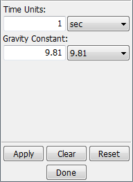
- Time Units
Enter/Select time units.
- Gravity Constant
Enter/Select gravity constant.
This interface is used to display normal vectors for any element in the model.
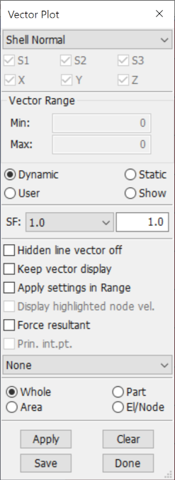
- S1/S2/S3
Switch on/off maximum principal vector.
- X/Y/Z
X/Y/Z-component of the vector.
- Min
Enter Minimum range value (Hit enter to accept entry).
- Max
Enter Maximum range value (Hit enter to accept entry).
- Dynamic
A set of min/max ranges is computed for each time state.
- Static
A constant min/max range is computed using all time states.
- User
Range set by user, enter min/max values above.
- Show
Show elements within the range entered above.
- SF
Select/Enter scale factor for vector plot.
- Hidden line vector off
Switch off hidden line for vectors.
- Keep vector display
Keep vector display after leaving menu.
- Apply settings in Range
Apply settings in Range dialog, say 'Actively element only', 'Region Min/Max' and 'ident min and max'.
- Display highlighted node vel
Display highlighted node velocity vector.
- Force resultant
Display resultant for visible force vectors.
- Prin. int.pt.
Display principal stress/strain for integration points in solid element.
- None
Find out the max(XVex) and min(XVen) throughout all states. Check only one S1, S2 or S3 if prin. stress/strain is selected.
- Whole
Apply vector plot to whole model.
- Part
Pick parts for vector plot.
- Area
Define an area for vector plot.
- El/Node
Pick an element or node for vector plot.
- Apply
Apply vector plot.
- Clear
Clear vector plot.
- Save
Save current vectors to file.
- Done
Exit Vector Plot interface.