VM-WB-MECH-112

VM-WB-MECH-112
Electrostatic Field Analysis of Quadpole Wires

Overview

Reference:	Any Basic Static and Dynamic Electricity Book
Solver:	Ansys Mechanical
Analysis Type(s):	Coupled Field Static
Element Type(s):	2D Plane Stress

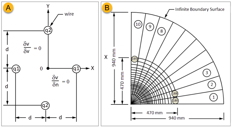
Test Case

Two wires of very small radius in a quadpole device system carry a positive charge q₁ and are located on the X-axis at positive and negative distances d from the origin O. Two wires of the same radius carry a negative charge q₂ and are located on the Y-axis at positive and negative distances d from the origin O. All wires extend in the Z-direction. Determine the electric potential V produced out to a radius of 470 mm measured from the origin O.

This problem is also presented in

VM49

in the Mechanical APDL Verification Manual.

Figure 173: A- Quadpole Wires Problem Sketch, B- Representative Finite Element Model

Figure 174: Ansys Mechanical Model

Materials Properties Tables

Material Properties	Geometric Properties	Loading
Relative Permittivity = 1	d = 25.4 mm	q₁ = 5E-7 q₂ = -5E-7

Material Properties

Geometric Properties

Relative Permittivity = 1

d = 25.4 mm

q₁ = 5E-7

q₂ = -5E-7

Analysis Assumptions and Modeling Notes

Two dimensional quad elements are used out to 470 mm of the radius. At this radius INFIN110 elements (also quad) with 470 mm radial length are used. The infinite boundary is therefore modeled to 940 mm, twice the radius of interest. Due to symmetry, only one quadrant (positive X and positive Y) is modeled with flux-normal boundary conditions at X = 0.0 and Y = 0.0. Only half of each wire in the first quadrant is included in the model by specifying one-half the charge magnitudes of q₁ and q₂.

Figure 175: A- Imported Mesh (CDB), B- Physics Region

The CDB file is imported using External Model. The Electric definition must be set to Charge for an active, pure electrostatic effect. The electric charge is applied to the nodes at distance d shown in the quadpole wire sketch. The following commands are used to define the infinite boundary conditions.

Commands to define infinite BC:

*get,attrmax,etyp,,num,max !attrmax = HIGHEST NUMBERED ATTRIBUTE ID IN MODEL
/prep7
ET,attnnax+1,INFIN110,1
keyop,attrmax+1,6€,1
r,2

csys,1
esel,s,cent,x,.47,.94
csys,0
emodif,all,type,attrmax+l
emodif,all,real,2
esel,all

cmsel,s,BC
SF,ALL,INF ! FLAG THE EXTERIOR FACE OF INFIN110 AT
allsel,all

/SOLU

Note: Since 4-node and 8-node elements are used together, the infinite element domain must be meshed before the finite element domain to force the element faces to drop their midside nodes at the interface of the finite and infinite element domain.

The finite element model uses a single 8-node, 2D quadrilateral element (PLANE121) and the INFIN110 element.

Results Comparison

The Ansys Mechanical results are compared with target specified in the reference.

V (Volt)	Target	Mechanical	Ratio (%)
At angle 0°	105.05	105.79	0.7
At angle 9°	99.90	100.62	0.7
At angle 18°	84.98	85.589	0.7
At angle 27°	61.74	62.184	0.7
At angle 36°	32.46	32.692	0.7
At angle 45°	0.00	0.00	0.0
At angle 54°	-32.46	-32.692	0.7
At angle 63°	-61.74	-62.184	0.7
At angle 72°	-84.98	-85.589	0.7
At angle 81°	-99.98	-100.62	0.6
At angle 90°	-105.05	-105.79	0.7