Equations of Motion for Rigid Bodies

Many methods are available to derive the equations of motion, such as Newton Euler equations, Gibbs-Appell equations, and Lagrange equations.

The combination of Gibbs-Appell equations with generalized velocities is often referred to as Kane's equations [KAN61]. Kane's equations are used for this example.

Open Loop Equations of Motion

The positional variation of a point M_k on body k is written as a reduction point using the origin of the body O_k :

(5–17)

Similarly, the translational acceleration of point M_k can be expressed using reduction point O_k :

(5–18)

The virtual work of the acceleration can be formed and integrated over body k, and summed over the bodies as follows:

(5–19)

The integration over the body leads to integrating quantities as follows:

(5–20)

These terms can be easily pre-calculated as follows:

(5–21)

In this equation, M_k stands for the mass of body k, and G_k stands for the center of gravity of that body. Other terms lead to:

(5–22)

where v is a constant vector. Those terms can be expressed as a function of the inertia tensor of body k.

Similarly, the virtual work of external distributed forces is computed as follows:

(5–23)

Finally, the open loop equations of motion lead to the following algebraic system:

(5–24)

Both the mass matrix M and the force vector F are dependent on the geometric variables and time t. The force vector is also a function of the generalized velocities.

(5–25)

When the mass and inertia properties of a rigid body are not constant, the force vector includes some additional terms dependent on the mass matrix time derivatives .

Equations of Motion with Flexible Bodies

Assuming that body k is flexible, the variation of the position of a point M'_k on body k is written, using the origin of the body O_k as a reduction point:

(5–26)

Similarly, the translational acceleration of point M'_k can be expressed using a reduction point O_k

(5–27)

As in the case of rigid bodies, the virtual work of the acceleration can be formed and integrated over body k, and summed over the bodies:

(5–28)

In presence of flexible bodies, the equations of motion are modified by 2 sets of terms:

Please refer to [SHA13] for more detailed information about the equations of motion.

Because the equilibrium is written on the current (deformed) configuration, the mass matrix and right hand side depend on the flexible degrees of freedom. To avoid having to go back to the finite element model to compute these integrals, these terms are decomposed over a basis of invariant terms, which are computed only once in the generation pass.

These invariants are expressed below. These terms are approximated using a lumped mass approach.

(5–29)

(5–30)

(5–31)

(5–32)

(5–33)

(5–34)

Where the Φ(i) are the Component Mode Synthesis base vectors.

Closed Loop Equations of Motion

When the model has some closed loops, not all joints can be treated as topological joints, thus requiring constraint equations to be added to the system. These constraint equations are usually written in terms of velocities as follows:

(5–35)

Each kinematic joint generates up to six of these equations, depending on the motion direction that the joint fixes.

To be introduced in the equations of motion, a time derivative of these equations must be written as follows:

(5–36)

The equations of motion for the closed loop system become:

(5–37)

Subject to:

(5–38)

An additional scalar variable λ (called a Lagrange Multiplier) is introduced for each constraint equation. These constraint equations are introduced in the algebraic system, which then becomes:

(5–39)

M, B, F, and G can be formed from a set of known geometric variables and kinematic variable values. The above system can be resolved, providing both accelerations and Lagrange multipliers λ.

These Lagrange multipliers can be interpreted as constraint forces, equivalent to the amount of force needed to prevent motion in the direction of the constraint equations.

Redundant Constraint Equations

The system matrix shown in Equation 5–39 has size n+m where n is the number of degrees of freedom, and m is the number of constraint equations in B. The mass matrix M is usually positive-definite, but the full matrix including the constraint equation will retain that property only if there are no redundant constraint equations in B.

The constraint equations are applied to the piston/crankshaft system shown below to demonstrate how the B matrix can contain redundant constraint equations.

Figure 5.10: Crankshaft Mechanism

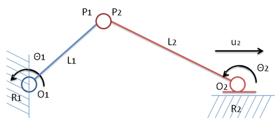
The revolute joint between point P1 on body 1 and point P2 on body 2 generates five constraint equations. For the sake of simplicity, these equations are written below in the global coordinate system, even if it is not always possible in general cases. The equations are:

These equations must be projected on the degrees of freedom. This is achieved in the code by writing the shape functions on each body on points P1 and P2:

(5–40)

(5–41)

and:

(5–42)

(5–43)

Replacing the velocities in the five constraint equations leads to:

The five equations above only generate two nontrivial constraints. The third equation indicates that the mechanism cannot shift along the z axis. It also indicates that the mechanism cannot be assembled if the z-coordinate of O₂ and O₂ are not the same. Similarly, the fourth and fifth equations indicate that the orientation of the axis of the revolute joint in P1/P2 is already entirely dependent on the axis of the two other revolute joints. A manufacturing error in the parallelism of the axis would result in a model that cannot be assembled. As such, this system is redundant.

Because introducing the five equations into Equation 5–39 would make the system matrix singular, some processing must be done on the full set of equations to find a consistent set of equations. Equations that are trivial need to be removed, as well as equations that are colinear. An orthogonalization technique is used to form a new set of equations that keep the matrix invertible. The matrix is decomposed into two orthogonal matrices, B_f and R:

(5–44)

where the [B_f] matrix has a full rank and [R] is a projection matrix. This matrix can then used in Equation 5–39:

(5–45)

Joint Forces Calculation

A benefit of using Kane’s equations and relative parameters is that joint forces in topological joints are eliminated from the algebraic system. Joint forces can be calculated explicitly by writing the dynamic equilibrium of each body recursively, starting from the leaves of the tree associated with the connection graph, with the unknown being the body parent joint’s forces and torque.

When the system has redundancies, that is, the [B] matrix does not have a full rank, some forces cannot be calculated. In the crankshaft example, no information is available in the forces developing in the revolute joint in P1/P2 in the z direction, and the moments cannot be calculated in this joint. These values will be reported as zero, but it is recommended that you avoid such situations by releasing some of the degrees of freedom in the system.