We assume here that the body is not rigid anymore, but undergoes small elastic deflections.

To define the position of a point of body k, we use a floating reference rigid body and define a small displacement vector between the point and its reference position on the floating reference body.

Figure 5.9: Flexible Bodies Kinematics

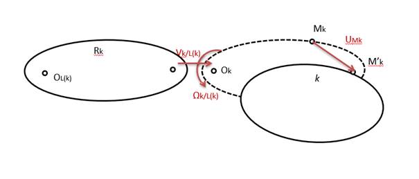
With the assumption of small deflections and elastic behavior, sub-structuring can be used to reduce the flexible body to a small set of DOFs. We will define a set of generalized coordinates q_i such that:

The global position of M' becomes:

(5–15)

The global velocity of M' is expressed by:

(5–16)

Compared to the rigid case, the translational shape functions are modified to be expressed at the flexible point location, and the flexible generalized coordinates now contribute to the shape functions.

The basis of vectors [N] is obtained using a Component Mode Synthesis analysis with Fixed Interfaces (see Component Mode Synthesis (CMS) in the Theory Reference for more details). Master nodes are created for each joint connected to the condensed part. The internal modes and attachment modes Φ are orthogonalized to form the N basis.

The point O_k can be any point in the condensed part. However, in practice, it can be either on a joint or on the center of gravity of the condensed part.