


This section describes in detail the major features and functions of BladeGen. The following sections are included.
The Meridional Profile is primarily determined by a set of curves (Hub, Shroud, Inlet, and Outlet). This data is modified with Leading and Trailing Edge Curves (and other Meridional Control Curves) to describe an interpolation surface or grid in axial (Z) and radial (R) coordinates vs. streamwise (U) and spanwise (V) positions. This interpolation grid is used when defining the layers that the Meridional Profile stores, which are referenced by the Angle, Thickness, and Prs/Sct Curves (for their position) and used to define the location of output data sets (See User/Data Interaction Summary ).
Beginning with version 4.1, here are two Meridional Profiles. The Design Meridional Profile is always required and is referenced from the Working Views to define the blade design. An optional Trim Meridional Profile has been added that allows a totally separate set of curves to be used and can be selected to be used for output.
Both Meridional Profiles are displayed in the Meridional View. The display of the two Meridional Profiles is controlled by Meridional View Popup Menu commands.
The following topics are discussed:
The Meridional View’s Popup Menu contains a section for the control of the Meridional Profile. By default, the Meridional View displays the Design Profile (which was previously the only profile available).
If the user desires to use a Trim Profile, the first step is to create one from the current Design Profile using the Meridional Profile | Create Trim Profile popup menu command. The user will be requested to specify the number of uniformly spaced spanwise layers which are to be created. The Trim Profile will be created using the first and last Layers defined for the Design Profile.
Once the Trim Profile has been created, there are several options and operations that become available.
The user can control which (or both) definition is to be displayed in the Meridional View using the Meridional Profile | Show Design Profile, Meridional Profile | Show Trim Profile, and Meridional Profile | Show Other Profile popup menu commands.
The user can modify the curves and layers which it contains using the same options that are available for the Design Profile.
The user can select which Meridional Profile is to be used when exporting using the Output | Use Design Profile or Output | Use Trim Profile menu commands.
The user can delete or recreate the Trim Profile using the Meridional Profile | Delete Trim Profile and Meridional Profile | Recreate Trim Profile popup menu commands.
The following topics are discussed:
The Meridional Control Curves are used to control the meridional interpolation grid. This grid is used to create layers and control spanwise interpolation of the other Working Views.
BladeGen now allows three modes of operation for Meridional Control Curves, as shown below. This enables the specification of geometry that was previously troublesome or even impossible. All three modes use the Inlet, Leading Edge, Trailing Edge, and Outlet Curves and add control curves at break points in the hub and shroud curves.
Minimal - The Minimal mode does not add additional control curves. It reproduces the interpolation grid of previous versions when the "Additional Control Curve" option was not enabled.
Normal - The Normal mode adds two predefined control curves at 35% and 65% of the blade’s meridional length. It reproduces the interpolation grid of previous versions when the "Additional Control Curve" option was enabled and is the default mode.
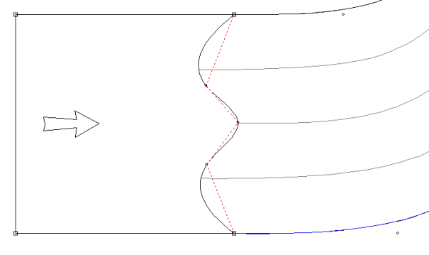
User-Defined - The User-Defined mode allows the user to add arbitrary control curves. Curves can be added at a mouse click or the user can request that a location be suggested when to improve the meridional interpolation. See the Meridional View Popup Menu for information on the additional menu commands available for this mode.
When in User Defined mode for Meridional Control Curves, the control curves are displayed as dashed lines (they are not displayed in other modes). In addition, the Meridional Control Curve sub-menu commands are enabled, which allow the following tasks to be performed.
The user can create additional control curves using the Suggest menu command. When selected, BladeGen searches the interpolation grid for the single worst orthogonal grid condition and, it if varies more than 30° from normal, creates a new control curve at that location.
The user can create control curves using the Insert menu command. This command specifies that a control curve should be created using the location of the next left mouse click. The curve is inserted between points on the hub and shroud that are closest to the specified point. Care should be taken to insure that the curve does not cross existing control curves (including the required Inlet, Leading, Trailing, and Exit curves). Invalid curves will not be created.
Control Curves can also be selected using the mouse and modified in all of the ways that the Leading and Trailing edge curves can be modified. This includes inserting points, splitting the curve into two or more segments, changing the segment type, and applying end treatments.
Selected Control Curves can be deleted individually using the Delete menu command.
Control Curves can be controlled by the end point positions using the Modify menu command. This command displays a Meridional Control Curve Dialog that can be used to create, delete, or modify control curves based upon the hub and shroud end point locations. The greatest usefulness of this dialog may be its ability to quickly delete a number of control curves quickly.
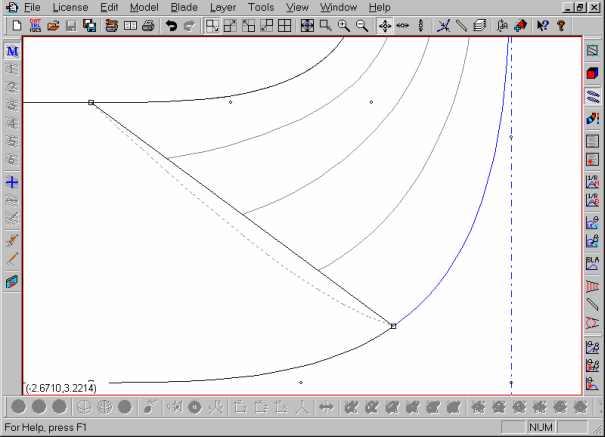
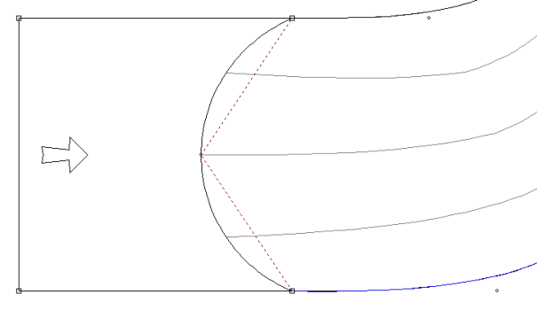
Previous versions of BladeGen attempted different ways of dealing with the specialized case where the user wants to have a spanwise curve that is a straight line in 3D space, but the hub and shroud points are at different theta locations. This is most often needed for a ruled element blade.
The difficulty comes from what happens to the curve when collapsed to the Meridional View. The straight 3D line forms a Hyperbola, as shown in the figure below as a dashed line.
There are now three modes available from the Use Hyperbolic Shape sub-menu of the Meridional View’s popup menu (shown below). These options allow the behavior to be specifically defined:
Never - The hyperbolic shape is never generated or used.
Ruled Element Only - The hyperbolic shape is used only for the Ruled Element angle definition spanwise interpolation mode.
Always - The hyperbolic shape is used for all angle definition spanwise interpolation modes.
As in previous versions, if a spanwise curve has more than one segment or the only segment has more than two points, then it is assumed that the user has specified the desired shape and the hyperbolic shape is not used.
The Use Hyperbolic Shape | Force Hyperbolic Shape menu command can be used to remove all interior points and extra segments from the spanwise curves, enabling the hyperbolic shape to be used.
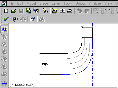
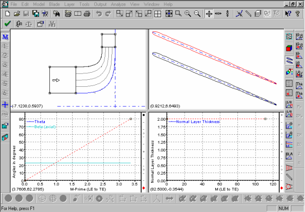
An arrow is displayed in the meridional view to indicate the direction of flow, as shown below. This is important because BladeGen requires the orientation of the blade in order to export to CFD grid generators, which need to have the fluid flow inlet and outlet defined. This direction can be reversed using the Tools | Reverse Flow Direction command and the Hub and Shroud Curves can be swapped with the Tools | Reverse Span Direction command.
A blue line is drawn in the Meridional View to indicate the current active layer for the Working Views and Blade-to-Blade View.
The following topics are discussed:
A layer (streamline) is defined as a meridional curve that represents surface of revolution. Angle, Thickness, and Prs/Sct Views display a single layer of the active blade and have a Layer Indicator to show location and provide an alternative layer navigation scheme (see Layer Coordination for details).
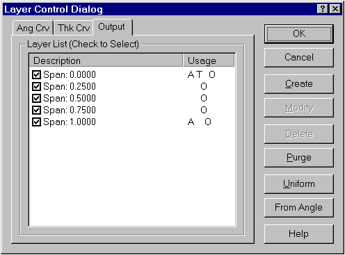
Layers are controlled (created, modified, and destroyed) using the Layer Control Dialog (Layer Control Dialog). This dialog can be accessed by selecting the Output | Output Layer Control... menu command or the Layer Control... menu command from a working view’s popup menu.
Related Topics
Trimming and Extending the Blade using Layers
This dialog provides access to the layers of the model. This dialog is re-used to specify which layers are to be used for the Angle, Thickness, Prs/Sct, and Output definition of the model, one at a time.
Also See:
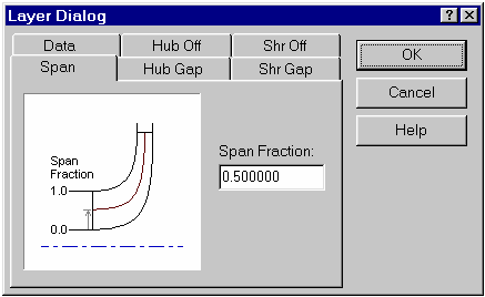
This dialog allows the user to select a layer’s type and set its parameters. This dialog is used for both initial setup of a layer and modification of a layers properties.
Select a tab to specify the layer type.
The Span tab selects the Span-wise Type and provides access to the parameters. Enter the location as a span fraction (normally 0 to 1, but values of -0.5 to 1.5 are accepted for Design Layers).
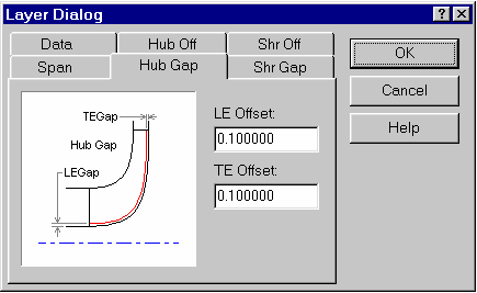
The Hub Gap tab selects the Hub Gap Type and provides access to the parameters. Enter a leading and trailing edge gap (in model units) into the spaces provided. The layer will be located using an offset vector normal to the hub. The magnitude of this offset vector at each point on the hub curve is determined by linear interpolation between the gap values entered for the leading and trailing edges. A positive value for either the leading or trailing edge gap implies a direction that is ’into the flow path’ (or towards the Shroud) for that gap.
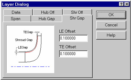
The Shr Gap tab selects the Shroud Gap Type and provides access to the parameters. Enter a leading and trailing edge gap (in model units) into the spaces provided. The layer will be located using an offset vector normal to the Shroud. The magnitude of this offset vector at each point on the shroud curve is determined by linear interpolation between the gap values entered for the leading and trailing edges. A positive value for either the leading or trailing edge gap implies a direction that is ’into the flow path’ (or towards the Hub) for that gap.
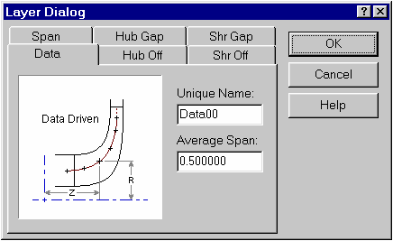
The Data tab selects the Data (User-Defined) Type and provides access to the parameters. Enter the approximate location as a span fraction (normally 0 to 1, but -0.5 to 1.5 for Design Layers). Once the layer has been created, it can be redefined in the Meridional View interactively using the same tools provided for other curves.
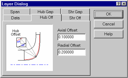
The Hub Off tab selects the Hub Offset Type and provides access to the parameters. This option creates a layer whose location from the Hub is defined by a constant offset vector. The radial and axial components of this vector are entered in the controls provided. A positive value for the radial or axial component implies a direction that is ’into the flow path’ (or towards the Shroud) for that component.
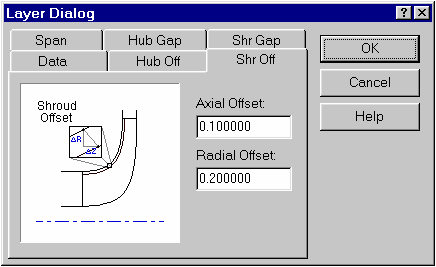
The Shr Off tab selects the Shroud Offset Type and provides access to the parameters. This option creates a layer whose location from the Shroud is defined by a constant offset vector. The radial and axial components of this vector are entered in the controls provided. A positive value for the radial or axial component implies a direction that is ’into the flow path’ (or towards the Hub) for that component.
All views display the Active Layer of the Active Blade. This layer is drawn in blue in the Meridional View and highlighted in the Layer Indicator of each of the Working Views, as shown below. If a Working View does not have a curve that references the Active Layer, a temporary curve is generated for display only.
The Layer Indicators display a point for each layer. The points are positioned by the layer’s span fraction with the bottom representing the hub (0% span) and the top representing the shroud (100% span). The current (active) layer is displayed as a red dot, other referenced layers displayed as black dots, and the remaining layers are displayed as gray dots.
There are (at least) three methods for selecting a layer (making it the Active Layer):
Move the mouse cursor into a Layer Indicator, position it over the desired point and press the left mouse button. The layer represented by the closest point will be selected.
Select the desired layer from the Layer sub-menu of the main menu or a Working View’s popup menu.
Move up and down the list of layers by pressing the ’+’ or ’-’ keys.
Layers can be created, modified, deleted, and referenced in a Working View using the Layer Control Dialog (Layer Control Dialog), which is also shown below. The dialog is displayed using the Output | Output Layer Control... menu command or the Layer Control... menu command from a Working View’s popup menu. The method used to access the dialog only determines which tab is initially selected.
The tabs of the dialog box change if a Trim Meridional Profile is defined. The "Output" tab is renamed to "Design" and a "Trim" tab is added.
The check boxes before the layer descriptions indicate how the layer is used. When the "Ang Crv", "Thk Crv", or "PSS Crv" tab is selected, checking a box creates a curve (of that type) that references the layer. When the "Output" or "Design" tab is selected, checking a box specifies that the layer is to be used for output. There are no check boxes in the "Trim" tab as all layers are used for output.
Note: When adding a layer reference to a view, make sure that the layer does not intersect other layers already referenced by that view. If an intersection does occur, a warning message will be displayed in the view and the situation should be corrected before proceeding.
Note: The Angle and Thickness views must reference at least one layer in their data definition. The Prs/Sct view must reference at least two layers (corresponding to the Hub and Shroud).
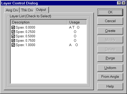
Layers can be flagged to specify where streamline data sets are to be constructed for output. The selection of layers for output is performed in the Layer Control Dialog (Layer Control Dialog) with the "Output", "Design", or "Trim" tab selected. The dialog is displayed using the Output | Output Layer Control... menu command or the Layer Control... menu command from a Working View’s popup menu.
The Purge button will remove all layers not referenced by any of the working views (even if they are flagged for output). Pressing the From Angle or From Prs/Sct button (mode dependent name) will cause all layers used in the Angle or Prs/Sct View to be flagged for output.
Note: At least two layers must be flagged for output.
It is not required that these layers be the same layers on which the blade is defined. Therefore, several operations can be performed by controlling which layers are exported.
Often a blade is defined by one or two layers in the Angle View or Prs/Sct View. However, if only two layers are output, many analysis and manufacturing programs may interpret the data differently than it was intended. This is also true for the internal throat surface calculation, which requires more than two output layers to function properly. It is, therefore, recommended that at least five layers be flagged for output so the blade is properly defined.
It was previously necessary to control which layers are flagged for output to trim or extend a blade in the spanwise direction. This functionality is still available for backward compatibility, but the Trim Meridional Profile provides a simpler and more powerful method of obtaining the same goal.
BladeGen uses the first and last layer flagged for output as the hub and shroud layers of the blade, respectively. This allows the user to trim or extend the blade by adding a layer at the desired trim location and making that layer the first or last layer flagged for output.
With the introduction of the Trim Meridional Profile, the practice of trimming or extending the blade by unselecting or adding hub and/or shroud layers is no longer required. The Trim Profile provides simpler and more powerful method of obtaining the same goal.
However, when the Design Profiles is selected for output, BladeGen still uses the first and last layer selected for output as the hub and shroud layers, respectively. This allows the user to trim or extend the blade by adding a layer at the desired trim location and making that layer the first or last layer flagged for output.
When a Trim Meridional Profile is created, the same scheme is used.
The following topics are discussed:
Most geometry operations in BladeGen involve direct manipulation of curves. All curves used in Working Views are multi-segmented (i.e. they are made up of one or more sub-curves) and share a common set of Segment Types and manipulation functions.
The following curve segment types are available:
Related Topics
The points that make up this segment type are joined by straight lines.
This segment type is often a good choice for the thickness curve and is also used as the default type when importing data into the Meridional View. It is not recommended for most other applications.
Please note that the segment type does not use the exact shape. Instead, a constant number of equally spaced points are used to create a spline that is used for interpolation. If the discontinuities are desired, the user should create break points.
This segment type is defined by a set of piecewise curves connecting the data points. These curves use an interpolation formula that is continuous through the second derivative. This derivative continuity is preserved at the junctions between piecewise curves, resulting in a smooth total curve that passes through all of the points.
This segment type forms the basis for many of the underlying operations within BladeGen, especially operations involving point conversions. It replaces the Lagrangian Spline curve used in previous versions.
This type of curve is defined by control points. It passes through the end points and is controlled by a set of intermediate points. The curve does not necessarily pass through the intermediate points. However, one of the properties of a Bezier curve is that the first point in from each end determines the angle at the end points.
Bezier curves are recommended for the design of a blade in the Meridional and Prs/Sct views, because they are both smooth in shape, and resistant to local curve distortions resulting from manipulation of the control points.
This segment type is defined by a polynomial curve, the coefficients of which are determined from a least squares fit to the data points in the segment. In general, this type of curve will not pass through any of the data points. However, BladeGen adds constraints to force the curve to pass through the end points. The order of the polynomial is specified by the user.
This type of curve is best suited to use where the data is "noisy" and some smoothing is required. It is the default curve type for imported Angle View curves.
Note: When BladeGen applies the end-point constraints it effectively predetermines some of the coefficients.
This segment consists of a 3-point circular arc. The arc is defined by the end points and either a fixed radius or a fixed angle. Editing of the middle point is performed using an Arc Parameters Dialog, created specifically for the task. A popup menu command can be used to flip the arc if required.
This type of segment is best suited for use in the Meridional View, where it is commonly used to define a leading or trailing edge. It is not available in the Angle and Thickness Views.
Note: Since this segment type uses only three points in its definition, changing to this type from any of the other segment types will result in a loss of the original data points.
The following topics are discussed:
The following curve operations are available in BladeGen:
These operations convert the segment to a different type while attempting to preserve the shape of the original segment. They are accessed by clicking the right mouse button in the appropriate view and selecting the Convert Points To option in the popup menu. The points may be converted to either Cubic Spline Points (points on the curve) or Bezier Control Points (points not necessarily on the curve).
The Convert Points to | Spline Curve Points... menu command converts the selected segment to a spline segment with a user-specified number of equally spaced points. BladeGen first creates new points on the original curve segment. It then fits a Cubic Spline through them to form the new curve segment.
The Convert Points to | Bezier Control Points... menu command converts the selected segment to a Bezier segment with the user specified number of control points. This is an approximation that attempts to reproduce the original curve by matching the end derivatives.
Most of the functions for this class of operations are contained within the Segment Operations popup menu, which can be displayed by clicking the right mouse button in the Meridional, Angle, Thickness, or Pressure/Suction views. The following options are available:
To start the point insertion mode:
Select the curve on which the new point will exist.
Click the right mouse button to display the popup menu.
Select Segment Operations | Insert Many Points from the popup menu.
Select the approximate locations using the left mouse button.
When finished:
Click the right mouse button to display the popup menu.
Select Segment Operations | Insert Many Points from the popup menu to terminate the point insertion mode.
Select the curve on which the new point will exist.
Click the right mouse button to display the popup menu.
Select Segment Operations | Insert Point from the popup menu.
Select the approximate location using the left mouse button.
Select the point to be deleted.
Click the right mouse button to display the popup menu.
Select Segment Operations | Delete Point from the popup menu.
Each view has a point location dialog box that is specific to its requirements. The angle and thickness views allow any one of four parameters to be used to specify the horizontal location of the point.
Select the desired point.
Click the right mouse button and select Segment Operations | Point Location... from the popup menu.
Enter the point coordinates.
The point location can also be edited by double-clicking with the left mouse button on a point. The Point Location Dialog will be displayed.
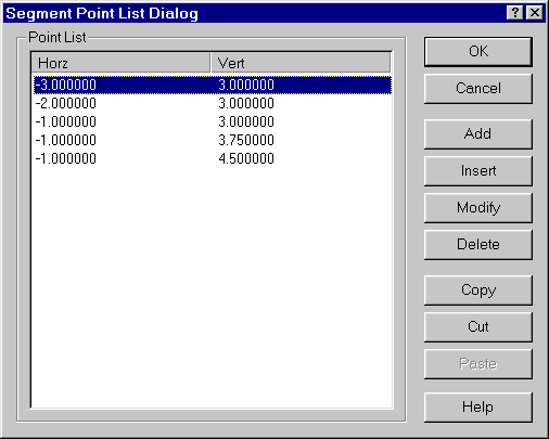
The entire point list can be edited by double-clicking the left mouse button between points. In this case, the Segment Point List Dialog will be displayed, as shown below. This dialog allows editing of groups of points. This dialog can also be accessed by invoking the Segment Operations | Segment Points... menu. See the Segment Point List Dialog for details on the functions available.
The following additional segment operations are available in BladeGen:
To split a segment at a point, select the desired point, click the right mouse button to display the popup menu, and select the Segment Operations | Split Segment at Point menu command or use the F3 key.
To join two segments at the point they share, select the point, click the right mouse button to display the popup menu, and select the Segment Operations | Join Segment at Point menu command or pressing the F4 key. If two different segment types are joined, the new combined segment will assume the type of the original upstream segment.
The Polynomial Order Dialog applies only to Best Fit Polynomial Segments. It is displayed when curve type is changed to a Polynomial or when the Segment Operations | Polynomial Order... popup menu command is selected.
The dialog box allows the user to specify the order of the polynomial. The value must be between (1+k) and (n-1-k). Where n is the number of points and k is determined by how many additional constraints are required. Two are required to insure the curve passes through the ends points, plus one for each end angle or tangency constraint.
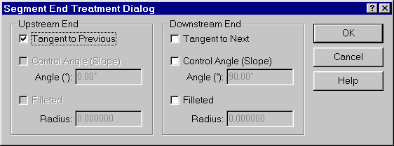
The Segment End Treatment Dialog, shown below, allows the user to apply additional constraints to both the upstream and downstream ends of the segment. It is accessed using the Segment Operations | End Treatment... menu command.
The dialog is not available in the Angle and Thickness Views, as only tangency can be specified. Instead the tangency is specified using the Segment Operations | Tangent to Previous and Segment Operations | Tangent to Next popup menu commands.
The details of the operation of the dialog and popup menu commands are available in the help.
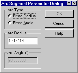
The Arc Segment Parameter Dialog, shown below, allows the user to specify the Arc Type (Fixed Radius or Fixed Angle) and then set the appropriate value (radius or angle). It is displayed by selecting an existing arc segment and performing one of the following operations:
Dragging the middle point.
Double-clicking on the middle point.
Depressing the right mouse button and selecting Segment Operations | Edit Arc Segment Parameter... from the resulting popup menu.
The Segment Operations | Flip Arc Segment menu toggles the arc segment between a concave and convex shape while preserving the existing radius or angle.
Reading Points from a File
The locations of all points on a curve segment can be defined by reading a file. Select the desired curve or segment, click the right mouse button to display the popup menu, and select the Segment Operations | Read Segment Points... menu command.
Saving Points to a File
The locations of all points in a curve segment can be saved to a file. Select the curve or segment, click the right mouse button to display the popup menu, and select the Segment Operations | Save Segment Points... menu command.
Curve Segment File Format
The first number in a curve segment file represents the total number of points. This is followed by the coordinates for each point (horizontal and vertical - one coordinate pair for each line) separated with a space, tab, and/or comma. The values must be in the dimensions displayed for the curve. If the curve is an angle curve, the angle must be in radians.
|
File Format Description |
Example File |
|---|---|
|
{number of points} |
5 |
|
{horizontal}{vertical} |
1 1 |
|
{horizontal}{vertical} |
1.0001e1, 2 |
|
: |
1.0003, 3 |
|
: |
1.1 5 |
|
: |
1.3, 6 |
BladeGen provides two options for translating an entire curve. These options are only available for curves in the Meridional View and are accessed by depressing the right mouse button in the view and selecting the Move Curve sub-menu from the resulting popup menu.
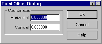
Move Curve | by Offset
This menu command displays a Point Offset Dialog, as shown below. This dialog prompts for both a horizontal and vertical distance. The entire curve will be offset by this vector.
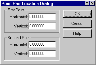
Move Curve | Intersect Two Points
This menu command displays a Point Pair Location Dialog, as shown below. This dialog prompts for the horizontal and vertical coordinates of two points. BladeGen will calculate an offset vector designed to move the curve as close as possible to both points. This offset vector will be displayed for confirmation in a Point Offset Dialog. The user may then either complete the operation by clicking OK or abort the operation by clicking Cancel.
To switch to a different segment type:
Select a segment with the mouse button.
Depress the right mouse button and select the Segment Type option from the resulting popup menu.
Select the desired segment type from the displayed list.
Note that this is different than performing the point conversion operations described above, because the shape of the original curve is not necessarily preserved. The new curve type uses the original set of points directly, even though it may interpret those points differently than the old curve type.
For example, when switching from a Bezier Curve to a Cubic Spline Curve, the new spline curve is simply fit through the original Bezier control points. This is different than using the Convert Points to | Spline Curve Points... function where BladeGen would first generate new points on the Bezier Curve and then fit a spline through them.
This section describes a class of functions that apply to the overall model or blade system. These functions are accessed using the Model menu.
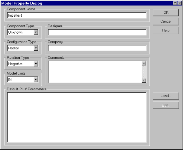
Users can assign various model properties within BladeGen using the Model Property Dialog, shown below. These properties are stored in the model and are used for some of the export options. These include a description of the component, the length units, the name of the designer and company, and a comment field. Access is also provided to the ’Plus’ parameters through the Load and Edit buttons.
If you transfer the geometry to BladeEditor, the Component Name serves to name the resulting BladeEditor blade.
The initial operating mode of a model is determined by the type of component selected in the Initial Meridional Profile Dialog or the mode assumed by the file type.
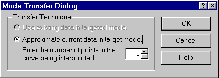
Users can change between operating modes by using the Model | Mode | Ang/Thk Mode... or Model | Mode | Prs/Sct Mode... menu commands. These commands display the Mode Transfer Dialog shown below, which, when transitioning between Angle/Thickness and Pressure/Suction Mode, allows the user to select how the conversion is to be made.
The first conversion option is to return to the data that already exists in the targeted mode, ignoring any changes made in the current mode. This option is disabled if there is no valid data in the targeted mode.
The second option transfers an approximation of the data in the current mode into the targeted mode, using the number of points specified for the curves.
BladeGen offers two options for calculating spanwise locations for layers or streamlines.
The Model | Spanwise Calculation | Geometric command specifies that the spanwise location is calculated based on geometric distance between hub and shroud. This option creates layers that are evenly spaced in the Meridional View.
The Model | Spanwise Calculation | Area Weighted command specifies that the spanwise location is calculated based on the flow path area. This option creates layers that represent the area fraction. For example, a span layer at 0.2 has 20% of the flow passage area ’below’ the curve and 80% ’above’ the curve.
The coordinate system used for design can be controlled using the Model | Coordinate System Orientation | Right-handed and Model | Coordinate System Orientation | Left-handed menu commands. These commands only affect the interpretation of the angle view data. Output is always converted to a right-handed coordinate system.
The following settings control various parameters in the Angle/Thickness Mode:
Beta Definition - The user has the option to define the angle Beta from either the axial direction or the tangential direction. These options are specified using the Model | Ang/Thk Beta Definition | Beta from Axial and Model | Ang/Thk Beta Definition | Beta from Tangential menu commands.
Data Direction - This option specifies the direction in which the Angle/Thickness data will be displayed, either from leading edge to trailing edge or from trailing edge to leading edge. The direction is selected using the Model | Ang/Thk Data Direction | From LE to TE and Model | Ang/Thk Data Direction | From TE to LE menu commands.
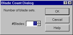
Select the Model | Number Blades Sets menu command or the ![]() toolbar button to specify the main blade count for the model. This will open a Blade Count Dialog, shown below, where the number of blade sets can be entered. Press OK to complete the operation or Cancel to abort the operation.
toolbar button to specify the main blade count for the model. This will open a Blade Count Dialog, shown below, where the number of blade sets can be entered. Press OK to complete the operation or Cancel to abort the operation.
In BladeGen, all curves (meridional curves, angle curves, thickness curves, and so on) are tessellated, yielding piecewise linear approximations. The point spacing on a tessellated curve is determined by recursively subdividing the curve until the maximum normal distance between the curve segment and its straight-line approximation falls below the specified value.
Tessellation points are used for display, but more importantly, they are also used in the calculation of blade geometry. The maximum allowed curve error affects:
The smoothness of curves displayed on the screen.
The accuracy of the BladeGen model, including point output.
The default value for the maximum allowed curve error is established when the model is initially created; the value is typically equal to 0.001 multiplied by an edge length of a bounding box of the meridional curves.
You can adjust the maximum curve error value using the Model | Maximum Curve Error... menu command.
This section describes parameters and functions that apply to a single blade. They are accessed using either the Blade menu or the blade toolbar.
BladeGen has the ability to design with splitter blades. Splitter blades are blades positioned between main blades for additional flow control. Splitter blades can be dependent on the main blade for their angular and thickness definitions or have their own, independent, definitions.
Like layers, BladeGen has one active blade at a time. Most views display only the data pertaining to the active blade. Only the Blade-to-Blade and 3D Views display all blades.
The following topics are discussed:
Each blade is defined by a series of parameters, accessible from a single Blade Property Dialog (shown below). Individual parameters, previously accessed from individual dialogs, are now accessed by selecting the appropriate tab. See Blade Property Dialog for more information.
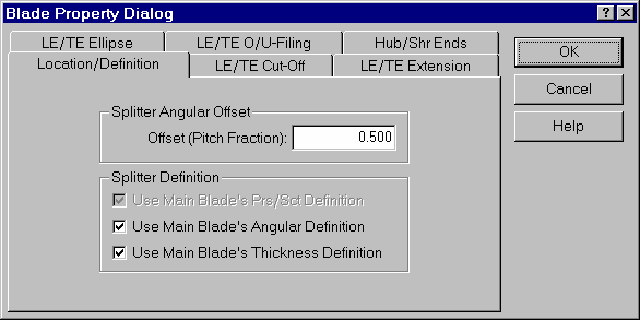
Splitter blades are added using the Blade | Add Splitter... menu command or the ![]() toolbar button. The Blade Property Dialog (Blade Property Dialog) will be displayed to allow the specification of the new blade’s parameters. The Location/Definition tab of this dialog box can used to specify whether the splitter uses the main blade’s Angle or Thickness Definition, and the offset of the splitter (expressed as a pitch fraction).
toolbar button. The Blade Property Dialog (Blade Property Dialog) will be displayed to allow the specification of the new blade’s parameters. The Location/Definition tab of this dialog box can used to specify whether the splitter uses the main blade’s Angle or Thickness Definition, and the offset of the splitter (expressed as a pitch fraction).
The current splitter blade can be deleted using the Blade | Del Splitter menu command or the ![]() toolbar button. To prevent accidental deletion of data, the user will be prompted for confirmation.
toolbar button. To prevent accidental deletion of data, the user will be prompted for confirmation.
The user can select the blade to be displayed by selecting the appropriate command from the Blade sub-menu or by pressing one of the toolbar buttons shown below.
![]() Main Blade
Main Blade
![]() Splitter1
Splitter1
![]() Splitter2
Splitter2
![]() Splitter3
Splitter3
![]() Splitter4
Splitter4
![]() Splitter5
Splitter5
![]() Splitter6
Splitter6
BladeGen offers several options for controlling the spanwise distribution of angle and thickness values. These options can be displayed by clicking the right mouse button in the Angle or Thickness View and selecting Spanwise Distribution Type sub-menu from the resulting popup menu. Note that it is allowable for the Angle View to have a different Spanwise Distribution type than the Thickness View. The following Spanwise Distribution types are available:
The General Distribution is the default Spanwise Distribution type. The parameter of interest (angle or thickness) is defined by curves on defining layers that use various meridional coordinates from those layers. Since these layers may have arbitrary shapes that don’t necessarily correspond to true streamlines, BladeGen must first convert their coordinates to "true" meridional coordinates (consistent with the meridional interpolation grid) before using them to compute the parameters to generate a blade.
The Ruled Element Spanwise Distribution type is only available in the Angle View.
In a ruled element blade, the angular location is defined by a straight line drawn in 3D space between points at the span location on the hub and shroud. The hub and shroud curves are the principal curves. They control the generation of all other defining curves. Thus, the hub and shroud curves are the only curves that the user can modify in the Spanwise Distribution type.
When one of the defining curves is updated from the hub curve, it obtains its location by the intersection of the surface of revolution generated using the meridional streamline and the lines drawn between corresponding pairs of points on the hub and shroud. Once this update occurs, a conversion is made to "true" meridional coordinates using the same method as in the general Spanwise Distribution type.
It is important to specify enough defining layers to adequately describe the geometry of interest. In most cases, 5 layers are sufficient.
Note: This option should be combined with the Hyperbolic Shape of Spanwise Curves (Hyperbolic Shape of Spanwise Curves ) option to produce the classic "Ruled Element" blade.
In an axial element blade, the parameter of interest (angle or thickness) depends exclusively on radial position (R) at each span location. The hub curve is the principal curve; it controls the curves for all of the other defining layers. Thus, the hub curve is the only curve that the user can modify in this Spanwise Distribution type. When a defining layer curve is updated from the hub curve, it obtains its parameter (angle or thickness) at a given meridional position by using an axial projection from the hub curve. Once this update occurs, a conversion is made to "true" meridional coordinates using the same method as in the general Spanwise Distribution type.
When using axial element blades, it is important to specify enough defining layers to adequately describe the geometry of interest. In most cases, 5 layers are sufficient.
When this distribution type is used in the Thickness View, there is a menu command in the popup menu to specify a taper angle. The taper angle, which normally defaults to zero, is limited to guarantee a minimum thickness of 10% of the specified value.
In a radial element blade, the parameter of interest (angle or thickness) depends exclusively on axial position (z) at each span location. The hub curve is the principal curve; It controls the curves for all of the other defining layers. Thus, the hub curve is the only curve that the user can modify in this Spanwise Distribution type. When a defining layer curve is updated from the hub curve, it obtains its parameter (angle or thickness) at a given meridional position by using a radial projection from the hub curve. Once this update occurs, a conversion is made to "true" meridional coordinates using the same method as in the general Spanwise Distribution type.
When using radial element blades, it is important to specify enough defining layers to adequately describe the geometry of interest. In most cases, 5 layers are sufficient.
The following topics are discussed:
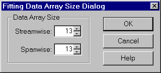
With this Spanwise Distribution type, the user generates an equation describing how the parameter of interest (theta or thickness) is distributed between the hub and shroud. Select the Spanwise Distribution Type | User-Defined menu command of either the Angle or Thickness Views to enable this option. The Fitting Data Array Size Dialog is displayed (see below) to allow the specification of the number of points that are to be collected and stored for use when fitting a User-Defined Spanwise distribution.
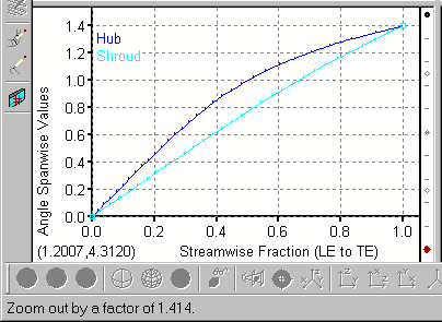
Once the fitting data has been collected, the view changes to the specialized spanwise view (shown below). The view initially displays the hub and shroud value curves which are required of every definition. A user-defined equation can then specified as described in Specifying the Equation . Any user-defined variables used in the equation are then also displayed in this view.
Several tools are provided to modify the data displays. First, as with the other Working Views, the user has access to all of the interactive curve modification tools. In addition, the user has the option of disabling the display of selected curves and scaling of values to maximize the utility of the view.
Related Topics:
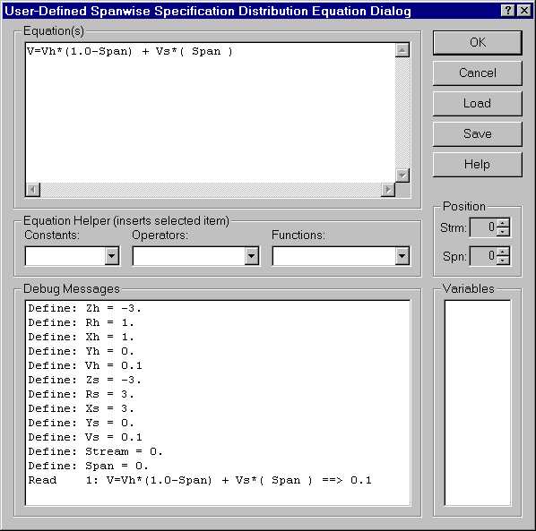
The equation can be defined by selecting the Edit Equation... command from the view’s popup menu. This will display the User-Defined Spanwise Specification Distribution Equation Dialog shown below.
Enter the equation into the "Equation(s)" control. The equation can be one or more lines. The "Equation Helper" controls can insert the selected Constant, Operator, or Function prototype into the equation.
There are several predefined variables that the equation can utilize. These are listed in below.
Table 9.5: Predefined Variables
|
Name |
Description |
|---|---|
|
Zh |
Z Location at the hub |
|
Rh |
Radial Location at the hub |
|
Xh |
X coordinate at the hub |
|
Yh |
Y coordinate at the hub |
|
Th |
Theta coordinate at the hub (Angle View only) |
|
Vh |
Value at the Hub |
|
Zs |
Axial coordinate at the shroud |
|
Rs |
Radial Location at the shroud |
|
Xs |
X coordinate at the shroud |
|
Ys |
Y coordinate at the shroud |
|
Ts |
Theta coordinate at the shroud (Angle View only) |
|
Vs |
Value at the shroud |
|
Stream |
Streamwise fraction ranging from 0.0 to 1.0 |
|
Span |
Spanwise fraction ranging from -0.5 to 1.5 |
|
V |
Returned value. Must be defined by the user equation. |
The equation must return the value of interest by assigning it to a variable call "V" (as shown in the equation below).
All user-defined variables (referenced but not defined) are listed in the Variables control. These variables are initially assigned a value of 0.1 (non-zero). These variables are actually curves which define the variable as a function of the stream fraction (ranging from 0.0 to 1.0).
The "Debug Messages" displays the result of evaluating the equation. It displays the predefined variables first (with a "Define:" statement) followed by each of the equation lines. The result of the evaluation is listed to the right of the equation. Only when this is error free is the equation valid.
Once the equations have been defined, the user may either view the differences between the new and original data, or have BladeGen attempt to adjust the equations to fit the new data to the original data. (The original data consists of the angle and thickness values that existed before the conversion to user-defined mode.)
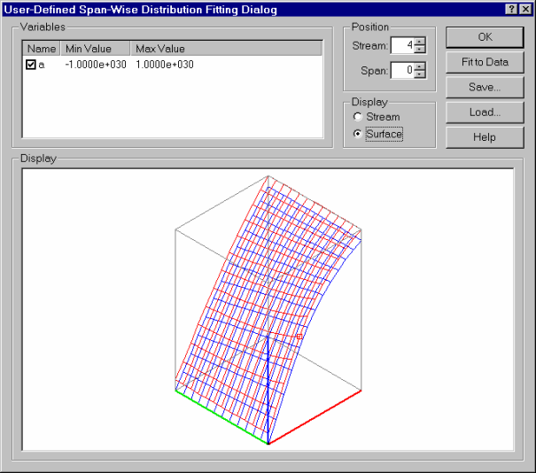
The variables can be fitted to the prior values by selecting the Fit to Data... popup menu command. The User-Defined Span-Wise Distribution Fitting Dialog, displayed below, provides access to data fitting functions and control of variable parameters when using a User-Defined Span-wise Distribution.
The user-defined variables are listed in the Variables control. Double-clicking on a variable displays the Variable Property Dialog which can be used to specify the minimum and maximum values for each variable. Each variable can be enabled or disabled (for fitting) using the check box in the Variables list.
The data is presented in the Display window (located at the bottom of the dialog) using one of two display modes - stream or surface.
In the stream display mode, the value (theta or thickness) is plotted as a function of span fraction at a given streamwise location. The original data (labeled "Data") is plotted in blue. The user defined curve (labeled "Curve") is plotted in red. The user can step through the streamwise and spanwise locations using the "Position" controls located in the upper right portion of the dialog.
In the surface display mode, the data is plotted in 3D. As in the "Stream" display mode, the original data is plotted in blue and the user-defined data is plotted in red. The axes drawn in the surface display are color coordinated shown in the table below.
Table 9.6: Surface Plot Axis Colors
|
Axis |
Color |
Description |
|---|---|---|
|
X |
Red |
Streamwise direction (x=0 represents the leading edge) |
|
Y |
Green |
Spanwise direction (y=0 represents the hub) |
|
Z |
Blue |
Data value (theta or thickness depending upon the view) |
When the Fit to Data button is pressed, the enabled user-defined variables are adjusted within their minimum and maximum values to attempt to find a better fit to the data. When completed, the result of the fitting process is displayed.
Pressing the OK button finalizes the fitting process. Press Cancel to abort the changes made and preserve the previous values of the user-defined variables.
The interpretation of the angle view data can be modified by using the Blade | Angle View Data Location | Side1, and Blade | Angle View Data Location | Side2 menu commands. The default assumption is that the angle view defines data on the mean line (the Blade | Angle View Data Location | Mean menu command). The Side1 and Side2 commands cause the data to refer to a side of the blade.
|
Option |
Description |
|---|---|
|
Mean |
is the default option and specifies that the theta values are for the location of the meanline. |
|
Side1 |
specifies that theta values locate Side1 of the blade. The thickness will be applied to specify the other side of the blade (at a larger theta value). |
|
Side2 |
specifies that theta values locate Side2 of the blade. The thickness will be applied to specify the other side of the blade (at a smaller theta value). |
Note: It is recommended that the Side1 or Side2 options be avoided if possible. These commands add another interpolation step to convert the data to mean line, so that the leading and trailing edge treatments can be applied and could result in reduced accuracy of the output.
The Blade | Thickness View Data Type sub-menu controls the meaning of the thickness data.
|
Option |
Description |
|---|---|
|
Normal to Meanline on Layer Surface |
This was previously called "Normal to Meanline" and is still the default. In this mode, the thickness specified in the thickness view is applied from a meanline point, normal to the meanline curve and on the layer surface (a surface of revolution). |
|
Normal to Camber Surface |
This option scales the specified thickness by the secant of the local blade lean angle in order to obtain the corresponding thickness measured on the layer surface. This has the effect of a normal-to-camber-surface thickness specification while keeping the computed thickness vector on the layer surface. |
|
Tangential on Layer Surface |
When this option is selected, the thickness vector is modified to be purely in the theta direction. |
Note: It is recommended that the tangential thickness option be avoided if possible. Currently all output uses data converted to normal thickness to prevent the leading and trailing edge treatments from being skewed. This could result in reduced accuracy of the output.
The Angle View allows the angular location of the blade to be specified using a number of methods. The user can select a method from the Angle View Popup Menu (Angle View Popup Menu). The following four types of angle definitions are available:
Angle Definition by End Angle
When defining the angle distribution of a blade using the End Angles option, only four points are used. They are the Theta and Beta at each end of the blade. Using these four points, the theta curve can be calculated using a third order polynomial. The beta values are then calculated from the derivative of the theta curve.
Angle Definition by End Angle with Zero Beta Slope
This option applies the End-Angle definition described above, with an additional restriction that sets the slope of the Beta curve to zero at the leading and trailing edges. The additional constraints make the polynomial fifth order.
Angle Definition by Theta Curve
When defining the angle distribution of a blade using the Theta Curve option, the user manipulates the theta curve directly. The beta values are then calculated from the derivative of the theta curve.
Angle Definition by Beta Curve
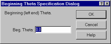
When defining the angle distribution of a blade using the Beta Curve option, the user manipulates the beta curve directly. BladeGen uses the beta curve values along with the leading edge theta value to calculate the remaining theta values. This calculation is performed using numerical integration. The leading edge theta value is zero by default, but can be modified using the "Beginning Theta Specification Dialog", shown below. This dialog is displayed by right clicking in the Angle View and selecting Theta @ Beginning... from the resulting popup menu.
The Auxiliary View is used to display various data sets describing the model and is automatically updated when modifications are performed in a Working View. The values displayed are calculated from the same data structures and functions that are used to output geometry for other purposes.
The Auxiliary View contents are controlled by the View menu (View Submenu) and the Auxiliary View Menu (Auxiliary View Menu), using the Auxiliary View Contents sub-menu. A new, independent Auxiliary View can be created by selecting the New Auxiliary View (B2B) menu command.
The following view types are available:
The following Auxiliary View Menu are available:
File Submenu - See File Submenu.
Layer Submenu - The Above command changes the displayed layer to the next layer above (by span). The Below command changes the displayed layer to the next layer below (by span). These commands allow rapid changes in the displayed layer, including layers which are not defining layers.
View Submenu - See View Submenu.
Window Submenu - See Window Submenu.
Help Submenu - Provides access to various help resources associated with this product. Also provides information about the point releases and software patches that are installed.
New - Create a new document.
Open - Open an existing document. The filename extension is used to determine the type of window in which it should be displayed.
Close - Close the active document (window).
Save - Save the active document. The Save command saves the document in the active window to disk. If the document is unnamed, the Save File As dialog box is displayed so you can name the file, and choose where it is to be saved.
Save As... - Save the active document with a new name. The Save As... command allows the user to save a document under a new name, or in a new location on disk. The command displays the Save File As dialog box. The user can enter the new file name, including the drive and directory. All windows containing this file are updated with the new name. If an existing file name is chosen, the user will be asked for confirmation to overwrite the file.
Compare... - Compare the current geometry to a saved blade geometry. The Compare... command displays the file selected in the File Open Dialog in the background (gray), behind the current model, for comparison. This allows the user to save a version of a model and then modify the current version with a visual comparison to the original model.
Export Submenu - See Export Submenu.
Print... - Print the active document. The Print... command prints the contents of the active window (or view). Use File | Print Preview... to see how the document will be laid out on printer pages. Use File | Print Setup... to select a printer, and to set printer options. Use File | Export | Report... to output a detailed report of a BladeGen model.
Print Preview - Display full pages. The Print Preview command opens a special window that shows how the active document will appear when printed. The preview window shows one or two pages of the active document as they would look when printed.
Print Setup... - Change the printer and printing options. The Print Setup... command displays the Printer Setup dialog box which allows you to select and configure the printer to be used to print documents in the application.
Preferences... - Display the User Preferences Dialog to allow the user to select some of the program defaults.
Recent File - Open a document from a selection of recently opened files.
Exit - Quits the application; prompts to save documents. If you have modified documents without saving, you will be prompted to save before exiting.
Text Data File... - Export a text description of the blade geometry to a ASCII text file. The Text Data File... command creates a formatted text file which includes R, Theta, Z, and normal thickness (Tn) for each of the layers in the specified directory.
RTZT File... - Export ’rtzt’ data to the specified file. The RTZT File... command create a generic ’rtzt’ file from the current model.
2D DXF Drawing Views... - Export 2D DXF drawing views as specified by the user. The 2D DXF Drawing Views... command creates a DXF file for each of the selected drawing views and tables to the specified directory. The Drawing View Dialog is displayed to control the output parameters. These files can then be imported into the users CAD system to generate a drawing of the blade geometry.
Pro/ENGINEER ibl File... - Export a Pro/ENGINEER ibl (wireframe only) datum curves to the specified file. The Pro/ENGINEER ibl File... command creates a wireframe Pro/Engineer ’ibl’ file which can be imported into Pro/Engineer using the Feature | Create | Datum | Curve | From File command. The file will include the hub and shroud curves and each blade, as defined on the output layers.
3D DXF File... - Export a 3D DXF wireframe to the specified file. The 3D DXF File... command creates a wireframe DXF file for inclusion into CAD drawings. The file will include the hub and shroud curves and each blade, as defined on the output layers.
3D IGES File... - Export a 3D model to the specified IGES file. The 3D IGES File... command creates a wireframe and optional surfaces in a IGES file for inclusion into CAD drawings. The file will include the hub and shroud curves and each blade, as defined on the output layers.
TurboGrid Input Files... - Exports a TurboGrid file set to the specified directory. The TurboGrid Input Files... command creates the hub, shroud, and profile files for Ansys TurboGrid in the specified directory.
ICEM TETIN File... - Export a CFX-HEXA file. The CFX-HEXA File... command exports an ICEM TETIN file for creation of a hexahedral mesh.
Toolbars Submenu - See Toolbars Submenu.
Arrange Views Submenu - See Arrange Views Submenu.
New Auxiliary View (B2B) - Display a new auxiliary Blade-to-Blade View of the current layer.
Auxiliary View Content Submenu - See Auxiliary View Content Submenu.
Ang/Thk Plot Horizontal Axis Submenu - See Ang/Thk Plot Horizontal Axis Submenu.
Layers for Plots of ’All Layers’ Submenu - See Layers for Plots of ’All Layers’ Submenu.
Main Toolbar - Show or hide the main toolbar. The Main Toolbar command toggles visibility of the main toolbar on/off.
Analysis Toolbar - Display Analysis Toolbar. The Analysis Toolbar command toggles the display of the Analysis Toolbar on/off.
Blade Toolbar - Show or hide the blade toolbar. The Blade Toolbar command toggles the display of the blade toolbar on/off.
Auxiliary Toolbar #1 - Show or hide auxiliary view toolbar #1. The Auxiliary Toolbar #1 command toggles the display of the auxiliary view toolbar #1 on/off.
Auxiliary Toolbar #2 - Show or hide auxiliary view toolbar #2. The Auxiliary Toolbar #2 command toggles the display of the auxiliary view toolbar #2 on/off.
3D View Toolbar - Show or hide the 3D View toolbar. The 3D View Toolbar command toggles visibility of the OpenGL toolbar on/off.
Status Bar - Show or hide the status bar.
Save Positions - Save the current positions for retrieval when the program starts. The Save Positions command saves toolbar positions for retrieval when the program starts.
All Four Views - Display all four views at the same size.
Top-Left View Only - Maximize the top-left view.
Bottom-Left View Only - Maximize the bottom-left view.
Bottom-Right View Only - Maximize the bottom-right view.
Top-Right View Only - Maximize the top-right view.
3D View - Change the auxiliary view to a 3D View
Blade-to-Blade View - Change the auxiliary view to the Blade-to-Blade View of the current layer.
Meridional Contour View - Change the auxiliary view to a Meridional Contour View of the current layer.
Meridional Curvature - Change the auxiliary view to a Meridional Curvature Graph.
Blade-to-Blade Curvature - Change the auxiliary view to the Blade-to-Blade Curvature Graph of the current layer.
Blade Lean Angle - Changes the auxiliary view to the Blade Lean Angle Graph of the hub and shroud.
LE/TE Theta - Change the auxiliary view to a LE & TE Theta Graph of the current layer.
LE/TE Beta - Change the auxiliary view to a LE & TE Beta Graph of the current layer.
LE/TE Parameters - Change the auxiliary view to a LE/TE Parameter Graph for the current blade. This view displays the all LE/TE Parameters vs. the % Span, including the elliptical ratio and over/under-filing parameters (where applicable).
Quasi-Orthogonal Area - Display the Quasi-Orthogonal Area Graph in the auxiliary view.
Airfoil Area - Change the auxiliary view to an Airfoil Area Graph. This graph plots the area in the blade loop of the Blade-to-Blade View at its mid-length span.
Maximum Diameter - Change the auxiliary view to a Maximum (Meridional) Diameter Graph. This data, combined with the throat data from the Blade-to-Blade view, can be used to determine the maximum spherical ball diameter.
Blade Information Table, Current Layer - Display the Information Table for the current layer in the auxiliary view.
Blade Information Table, All Layers - Display the Information Table for all of the defined layers in the auxiliary view.
Blade Angles, Current Layer - Display a Blade Angle Graph (Theta and Beta) for the current layer in the auxiliary view.
Blade Angles, All Layers - Display a Blade Angle Graph (Theta and Beta) for all of the defined layers in the auxiliary view.
Theta, All Layers - Display a graph of Theta for all of the defined layers in the auxiliary view.
Beta, All Layers - Display a graph of Beta for all of the defined layers in the auxiliary view.
Beta vs. Theta, All Layers - Display a graph of Beta vs. Theta for all of the defined layers in the auxiliary view.
Thickness, Current Layer - Display a graph of the blade thickness for the current layer in the auxiliary view.
Thickness, All Layers - Display a graph of blade thickness for all of the defined layers in the auxiliary view.
M-Prime Position - Display the current blade angle or thickness graph with the horizontal axis using the radius normalized meridional distance (M-Prime).
% M-Prime Position - Display the current blade angle or thickness graph with the horizontal axis using the percent of the radius normalized meridional distance (%M-Prime).
Meridional Position - Display the current blade angle or thickness graph with the horizontal axis using the meridional distance (M).
% Meridional Position - Display the current blade angle or thickness graph with the horizontal axis using the percent of the meridional distance (%M).
% Camber Length - Displays the current thickness graph with the vertical axis displaying the blade thickness as the percent of the total camber length and the horizontal axis displaying location as the percent of the total camber length.
Axial Loc (Z) - Display the current blade angle or thickness graph with the horizontal axis using the axial location (Z).
Radial Loc (R) - Display the current blade angle or thickness graph with the horizontal axis using the radial location (R).
All Layers - Specify that the data from all existing layers should added to ’All Layer’ plots.
Output Layers - Specify that only data from output layers should added to ’All Layer’ plots.
Defining Layers - Specify that only data from layers used to define the blade should added to ’All Layer’ plots.
New Window - Open another window for the active document.
Cascade - Arrange windows so they overlap. The Cascade command arranges all document windows from the top-left position of the application’s main window so that the title bar of each is visible.
Tile Horizontal - Arrange all document windows horizontally in a non-overlapping pattern.
Tile Vertical - Arrange all document windows vertically in a non-overlapping pattern.
Arrange Icons - Arrange icons at the bottom of the window.
The following topics are discussed:
The Blade-to-Blade view, shown below, combines the meridional, angular, and thickness descriptions of the blade along a streamline (called a layer). The blade is displayed as a function of the distance along the streamline in the meridional view and its angular position using one of three Coordinate Systems (Coordinate Systems ).
This view is displayed using either the View | Auxiliary View Content | Blade-to-Blade View menu command or the ![]() toolbar button (located by default on the right edge of the main window). See Blade-To-Blade View Popup Menu for details of the options and functions available in this view.
toolbar button (located by default on the right edge of the main window). See Blade-To-Blade View Popup Menu for details of the options and functions available in this view.
Layer Submenu - The Above command changes the displayed layer to the next layer above (by span). The Below command changes the displayed layer to the next layer below (by span). These commands allow rapid changes in the displayed layer, including layers which are not defining layers.
New Auxiliary View (B2B) - Display a new auxiliary Blade-to-Blade View of the current layer.
Auxiliary View Content Submenu - See Auxiliary View Content Submenu.
Coordinate System Submenu - See Coordinate Systems .
Show Points - Toggle the display of the defining points on/off.
Show Centroid - Toggle the display of the blade centroid on/off.
Show Throat(s) - Toggle the display of throat(s) on/off.
Show LE/TE - Toggle the display of the leading and trailing edges on/off.
Copy View Image/Data to Clipboard - Copy the Current View’s Image and/or Data to the Clipboard (in text, bitmap, or metafile formats). This allows transfer of data to reports, spreadsheets, and presentations for documentation of the blade design.
Zoom Fit - Zoom to fit the data within the current view.
The Blade-to-Blade view displays the shape of the blade on a surface of rotation that may or may not be cylindrical or planar. Therefore, a conformal coordinate system must be used to transform the 3D data into a 2D view. Several systems have been developed over the years, each with its strengths and weaknesses, as detailed below. The selection of one system over another is left to the user.
Note: See the section on BladeGen Definitions for the definitions of the variables used.
The selection of the coordinate system is performed using the Coordinate System sub-menu of the view’s popup menu. The following coordinate systems are available:
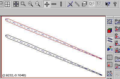
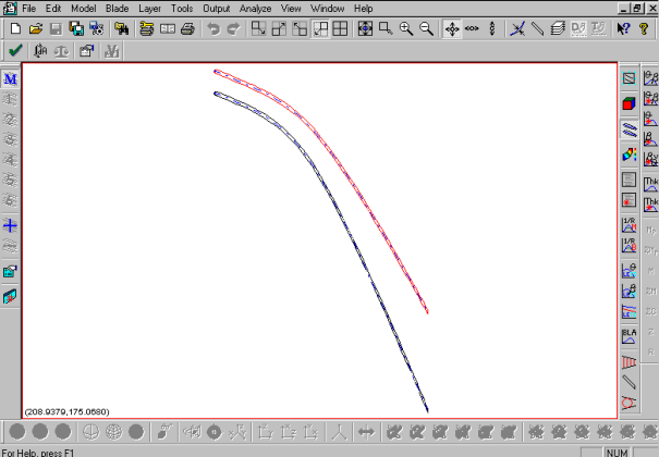
The M-Prime vs. Theta conformal coordinate system presents all of the blades in an angular shape preserving view, as shown below. However, because of the normalizing of the meridional distance with radius, the thickness of the blade is distorted.
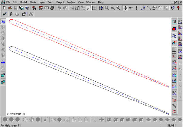
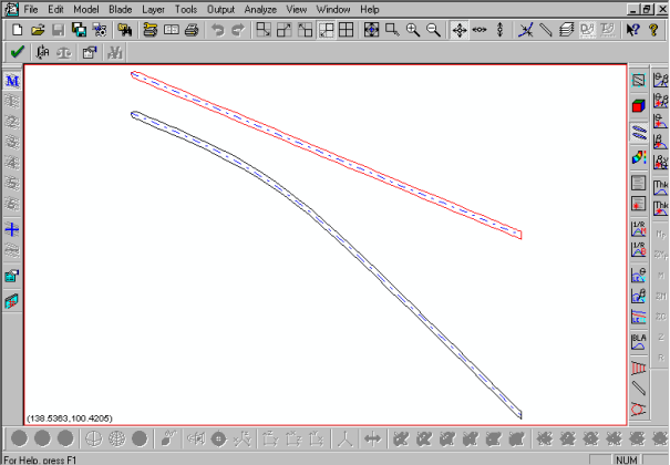
The M vs. R*Theta conformal coordinate system preserves the thickness of the blade, as shown below. However, the angular shapes of all blades are distorted.
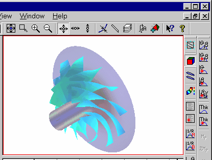
This view allows the user to visualize the model in three dimensions, as shown below. The model can be dynamically rotated, panned and zoomed to achieve the desired viewing perspective. With material (surface) visibility and clipping plane controls, the user can choose to view a subset of the model in greater detail. The user may also choose to view multiple blades by using the replicates controls. Like any other auxiliary view, the 3D view is automatically updated when a change is made in one of the working views. This view is displayed using the View | Auxiliary View Content | 3D View menu command or the ![]() toolbar button.
toolbar button.
The following display controls are available with the 3D view:
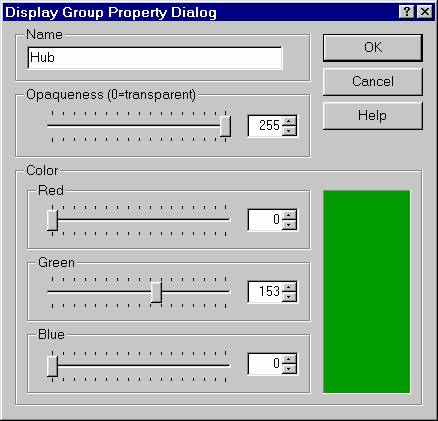
The Display Group Control... menu command controls which items are displayed in the 3D view. This command will display the Display Group Control Dialog shown below. Placing a checkmark in the box to the left of an item will cause that item to be displayed.
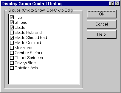
Double clicking on an item in the Display Group Control Dialog will invoke a Display Group Property Dialog for that item, as shown below. This dialog allows the user to set the following display attributes for the selected item:
Opaqueness - This controls the transparency of the item when the model is shaded. (0=transparent, 255=opaque).
Color - This will be the unshaded color of the item (i.e. the color of the item when the model is displayed in either Wireframe or Meshed mode).
Objects may be displayed in three different ways, as shown below. The desired view type can be selected in the view’s popup menu (using the Surface Display command) or by pressing a toolbar button.
Table 9.7: 3D View Display Options
|
Menu Command |
Button |
Description |
|---|---|---|
|
Wireframe |
|
Shows the curves that define the edges of the surfaces. |
|
Meshed |
|
Shows the surface mesh from which the shaded surfaces and volume mesh will be defined. |
|
Shaded |
|
Shows opaque surfaces defined by the surface mesh. |
In a BladeGen model of a cyclically symmetric blade system, only the geometry between a single set of periodic boundaries is stored. This geometry typically consists of a main blade and any associated splitters. Even though BladeGen does not store redundant geometry, it allows the user to visualize the entire blade system by using replicates. The table below lists the available commands for viewing replicates. These commands are accessed by using the Replication option in the view’s popup menu or by pressing the appropriate toolbar button.
Table 9.8: 3D View Replication Options
|
Menu Command |
Button |
Description |
|---|---|---|
|
Original Only |
|
Shows a single blade (and any splitters). This is the model stored in BladeGen and used for flow calculations. |
|
One Replica |
|
Shows two side-by-side blades. Useful to see how the individual blade models fit together. |
|
All Replicas |
|
Shows the entire blade system. |
Clipping planes allow the user to explore the inside of the model by clipping away parts of the view. There are six clipping planes available. To activate the clipping planes, use the Clip command in the view’s popup menu or the toolbar buttons. These provide options to toggle each plane on or off, select which plane to move with the mouse wheel, and open the Clipping Plane Property Dialog. With Windows NT and later, the selected clipping plane can be moved by depressing the mouse wheel and then rotating it.
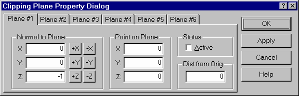
Each clipping plane can be customized with the Clipping Plane Property Dialog, shown above, which is accessed using the Clip | Setup menu command or the ![]() toolbar button. This dialog allows the user to specify the clipping direction (either by setting the components of a vector normal to the plane or by using one of the predefined direction options). It also allows the user to set the initial plane location, either by specifying the coordinates of a point on the plane or by setting a minimum distance from the origin. The clipping plane can also be activated and deactivated in this dialog.
toolbar button. This dialog allows the user to specify the clipping direction (either by setting the components of a vector normal to the plane or by using one of the predefined direction options). It also allows the user to set the initial plane location, either by specifying the coordinates of a point on the plane or by setting a minimum distance from the origin. The clipping plane can also be activated and deactivated in this dialog.
The clipping planes are initially defined as shown below.
Table 9.9: Clipping Plane Default Values
|
Plane No. |
Plane |
Side Displayed |
|---|---|---|
|
1 |
XY |
-Z |
|
2 |
YZ |
+X |
|
3 |
XZ |
+Y |
|
4 |
XY |
+Z |
|
5 |
YZ |
-X |
|
6 |
XZ |
-Y |
The viewpoint controls are provided to manipulate the orientation and position of the 3D View. A combination of keyboard shortcuts, menu commands, or mouse buttons are available. In addition, some of the menu commands are duplicated on the toolbars.
Table 9.10: 3D View Menu/Keyboard Equivalent Commands
|
Function |
Menu Command |
Keyboard Shortcut |
|---|---|---|
|
Positive rotation about X |
Rotate | X+ |
Ctrl + down arrow |
|
Negative rotation about X |
Rotate | X- |
Ctrl + up arrow |
|
Positive rotation about Y |
Rotate | Y+ |
Ctrl + right arrow |
|
Negative rotation about Y |
Rotate | Y- |
Ctrl + left arrow |
|
Rotate Counter-Clockwise |
Rotate | Z+ |
Shift + Ctrl + right arrow |
|
Rotate Clockwise |
Rotate | Z- |
Shift + Ctrl + left arrow |
|
Translate Right |
Translate | Right |
Shift + Right Arrow |
|
Translate Left |
Translate | Left |
Shift + Left Arrow |
|
Translate Up |
Translate | Up |
Shift + Up Arrow |
|
Translate Down |
Translate | Down |
Shift + Down Arrow |
|
Translate In |
Translate | In |
Ctrl + Shift + up arrow |
|
Translate Out |
Translate | Out |
Ctrl + Shift + down arrow |
|
Look down X axis |
Align | Along X |
x |
|
Look down Y axis |
Align | Along Y |
y |
|
Look down Z axis |
Align | Along Z |
z |
|
Isometric |
Align | Isometric |
i |
|
Flip (rotate 180 about Y) |
Align | Flip |
f |
|
Reset View |
Zoom | Fit |
Home |
|
Zoom Box |
Zoom | Box |
End |
The coordinates in the above table refer to screen coordinates where positive X is to the right, positive Y is upwards and positive Z is out of the screen. Positive rotation about a given axis is defined as counterclockwise when looking down that axis from its positive direction.
Table 9.11: 3D View Mouse Commands
|
Function |
Mouse Movement |
|---|---|
|
Rotate Model |
Drag with left mouse button pressed |
|
Translate Model |
Drag with right mouse button pressed |
|
Zoom & Spin Model |
Drag with both mouse buttons pressed |
|
Zoom |
Rotate mouse wheel (NT only) |
|
Scroll Clipping Planes |
Rotate mouse wheel with Shift pressed (NT only) |
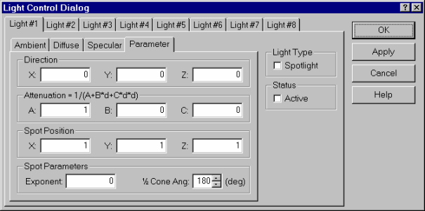
The 3D view allows up to eight lighting sources. The user may override the default parameters for these sources by using the Light Control Dialog shown below. This dialog is displayed by using the Light Control... popup menu command.
In the 3D view, the material properties control the display of the shaded surface. The Material Control Dialog, shown below, allows the user to set material properties (such as color and shininess) for these surfaces. The Material Control Dialog is displayed by using either the Front Material Def... or the Back Material Def... popup menu command.
BladeGen allows the user to specify different lighting properties on the front and back sides of a surface. (The front side is typically the side exposed to the flow path.) Use the Shaded Material Mode | Front/Back Unique popup menu command to select this option.
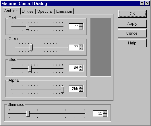
The Shaded Material Mode | Front/Back Same popup menu command forces both the front and back material properties to be the same. In this case, the Back Material Def... popup menu command will be disabled and both sides will use the properties of the front material.
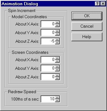
The animation capability of the 3D view allows the user to see the model rotating on the screen. To animate the model, select the Animate popup menu command from the view’s popup menu. The user can customize the way the animation is performed by using the Animation Dialog shown below. This dialog is displayed using the Animation Setup... popup menu command. The degrees of rotation per animation frame can be entered in either model or screen coordinates. The speed at which the frames will be shown can also be entered. However, the speed of the animation will ultimately be limited by the speed of the CPU and graphics card.
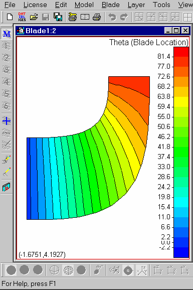
BladeGen allows the user to plot contours of Theta, Beta, Lean, or Thickness on the meridional profile, as shown below. This view can be displayed using the View | Auxiliary View Content | Meridional Contour View menu command or by pressing the ![]() toolbar button (located by default on the right edge of the main window).
toolbar button (located by default on the right edge of the main window).
The Contour view can display the following values: Theta (Blade Location); Beta (Blade Angle); Blade Lean Angle; Normal Thickness; and Modified Thickness (Includes Over/Under-Filing).
The user can select from several grid densities: Very Fine; Fine; Medium; and Coarse. These settings use predetermined point counts which are distributed using the lengths of the four edges of the blade.
See Contour View Popup Menu for details of the options and functions available in this view.
Blade Submenu - See Blade Submenu.
New Auxiliary View (B2B) - Display a new auxiliary Blade-to-Blade View of the current layer.
Auxiliary View Content Submenu - See Auxiliary View Content Submenu.
Theta (Location) Angle - Display a color contour plot of blade angle (Theta) in the Meridional View using the current interpolation grid density.
Beta (Blade) Angle - Display a color contour plot of blade angle (Beta) in the Meridional View using the current interpolation grid density.
Blade Lean Angle - Display a color contour plot of the blade lean angle in the Meridional View using the current interpolation grid density.
Normal Thickness - Display a color contour plot of blade thickness in the Meridional View using the current interpolation grid density.
Modified Thickness - Plot Modified (with Over/Under-Filing) Thickness Contours in the Meridional View. The Modified Thickness command selects the ’Enhanced Thickness’ data for display in the Contour View. The ’Enhanced Thickness’ is the blade thickness with any over/under-filing applied (but not the ellipse or cut-off).
Data Grid Density Submenu - Set the density of the grid used to interpolate contour data. When a contour plot is generated, blade data for the selected data type is extracted for each point in the interpolation grid. Contour boundaries are then generated by interpolating between the values at these data points.
Show Contour Lines - Show solid lines between contour levels.
Show Data Points - Show the points at which blade data is extracted for contour plotting.
Show Grid - Display the interpolation grid used to extract blade data for contour plotting. Each intersection in the grid represents a point at which blade data is generated.
Copy View Image/Data to Clipboard - Copy the Current View’s Image and/or Data to the Clipboard (in text, bitmap, or metafile formats). This allows transfer of data to reports, spreadsheets, and presentations for documentation of the blade design.
Zoom Fit - Zoom to fit the data within the current view.
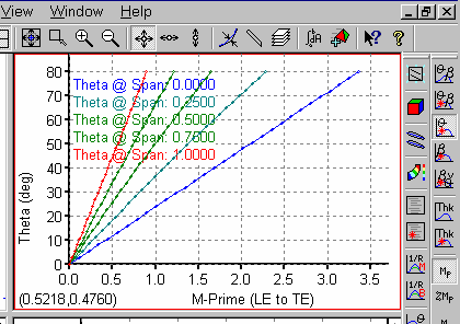
The graph view displays the selected data in an X-Y plot (as shown below) and is the workhorse of the Auxiliary Views. The graph type is selected using the View | Auxiliary View Content menu command or the Auxiliary Toolbars (displayed by default on the right edge of the window). See Graph View Popup Menu for details of the options and functions available in this view.
Fly-Over bubble help is provided for additional information on the points. The user can position the mouse cursor over a point and the bubble help will be displayed to describe these parameters. The bubble is removed when the user clicks a mouse button or moves the mouse over the bubble. For more information, see Hover Help .
Layer Submenu - The Above command changes the displayed layer to the next layer above (by span). The Below command changes the displayed layer to the next layer below (by span). These commands allow rapid changes in the displayed layer, including layers which are not defining layers.
New Auxiliary View (B2B) - Display a new auxiliary Blade-to-Blade View of the current layer.
Auxiliary View Content Submenu - See Auxiliary View Content Submenu.
Ang/Thk Plot Horizontal Axis Submenu - See Ang/Thk Plot Horizontal Axis Submenu.
Layers for Plots of ’All Layers’ Submenu - See Layers for Plots of ’All Layers’ Submenu.
Show Legend - Toggle the display of the legend on/off.
Show Points - Toggle the display of the data points on/off.
Show Comparison Curves - Toggle the display of the data curves from the comparison model on/off. These curves are darker in color and use a smaller marker to differentiate them from the other curves.
Number of Points... - Displays a dialog to allow the user to select the number of points displayed in the curves.
Swap Axes - Swap the horizontal and vertical axes of the selected graph.
Proportional Axes - Toggle the proportionality setting of the graph axes on/off.
Flip X Axis Direction - Flip the direction of the X Axis. When the Axis is flipped, the positive direction is reversed.
Flip Y Axis Direction - Flip the direction of the Y Axis. When the Axis is flipped, the positive direction is reversed.
Log X Scale - Toggle between Linear and Log (base 10) scaling on the horizontal axis.
Log Y Scale - Toggle between Linear and Log (base 10) scaling on the vertical axis.
Save Graph Data... - Save the data from the graph to the specified file. The Save Graph Data... command displays the File Save Dialog and saves the data in the current graph in the specified file. The file is comma delimited and can be read into Microsoft Excel(tm) or similar software.
Copy View Image/Data to Clipboard - Copy the Current View’s Image and/or Data to the Clipboard (in text, bitmap, or metafile formats). This allows transfer of data to reports, spreadsheets, and presentations for documentation of the blade design.
Zoom Fit - Zoom to fit the data within the current view.
BladeGen displays a number of data sets in the Graph View. The table below lists the current data sets.
|
Menu Command |
Button |
Description |
|---|---|---|
|
Meridional Curvature |
|
Meridional Curvature vs. Meridional Fraction |
|
Blade-to-Blade Curvature |
|
Blade-to-Blade Curvature vs. Meridional Fraction |
|
LE/TE Theta |
|
LE/TE Theta vs. %Span |
|
LE/TE Beta |
|
LE/TE Beta vs. %Span |
|
LE/TE Parameter Graph |
|
|
|
Blade Lean Angle |
|
Blade Lean Angle vs. %M The angle is measured between a constant-Theta plane and a line segment, where:
|
|
Quasi-Orthogonal Area |
|
Quasi-Orthogonal Area vs. Meridional Fraction |
|
Airfoil Area |
|
Airfoil Area vs. Span Fraction The airfoil area is the section area for the blade on a given span layer. It is calculated by numerical integration (trapezoidal rule) between the pressure and suction sides. |
|
Maximum Diameter |
|
Maximum Meridional Diameter vs. Meridional Fraction |
|
Blade Angles, Current |
|
Blade Angles (Current Layer) vs. Mp, %Mp, M, %M, Z or R |
|
Blade Angles, All |
|
Blade Angles (All Layers) vs. Mp, %Mp, M, %M, Z or R |
|
Theta, All |
|
Theta (All Layers) vs. Mp, %Mp, M, %M, Z or R |
|
Beta, All |
|
Beta (All Layers) vs. Mp, %Mp, M, %M, Z or R |
|
Beta vs. Theta |
|
Beta vs. Theta (All Layers) |
|
Thickness, Current |
|
Thickness (Current Layer) vs. Mp, %Mp, M, %M, %C, Z or R |
|
Thickness, All |
|
Thickness (All Layers) vs. Mp, %Mp, M, %M, %C, Z or R |
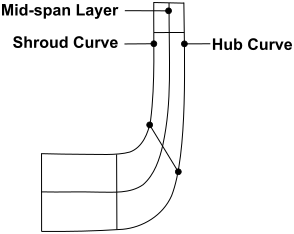
Blade and layer properties may be displayed in text format in the auxiliary view by using either of the following menu commands:
View | Auxiliary View Content | Blade Information Table, Current Layer
View | Auxiliary View Content | Blade Information Table, All Layers
These commands will generate a view similar to the one shown below. Additional throat data may be included in the view by selecting the Include Throat Calculation command from the view’s popup menu.
Note: Different information will be displayed in this view depending on whether the operating mode is Angle/Thickness or Pressure/Suction.
BladeGen provides a class of operations for performing global geometry modifications to the blade system. These operations are accessed through the Tools sub-menu and are described below.
|
Sub-Menu Command |
Description |
|---|---|
|
Scale Model... |
Scales the model by a specified factor. See Scaling the Model for more information. |
|
Shift in Z Direction |
Translates the model along the axis by a specified distance. See Shifting the Model in the Z Direction for more information. |
|
Flip Z Dimension |
Changes the sign of the axial (Z) dimension of all meridional points. |
|
Reverse Span Direction |
Swaps the hub and shroud curves for the model. |
|
Reverse Flow Direction |
Reverses the streamwise direction for the model by swapping the leading and trailing edge curves, inlet and outlet curves, and all cut-off or extension curves. |
|
Reverse Rotation Direction |
Reverses the sign of the theta values for the model. |
|
Zero Average LE Theta |
Attempts to minimize the value of theta on the leading edge of the blade. This is accomplished by calculating an average leading edge theta over all of the layers and offsetting every theta value in the model by this result. Note that this operation does not change the overall shape of the blade system. |
|
Zero Average TE Theta |
Attempts to minimize the value of theta on the trailing edge of the blade. This is accomplished by calculating an average trailing edge theta over all of the layers and offsetting every theta value in the model by this result. Note that this operation does not change the overall shape of the blade system. |
|
Blade Rotation Setup... and Rotate Blade |
Rotates the blade about an axis. See Blade Rotation Operations for more information |
|
Stack Blade on Centroid |
Aligns each blade layer’s centroids (in the tangential direction) to the hub layer’s centroid. The purpose of this operation is to modify the blade shape to reduce bending stresses under rotational loads. |
|
Create from Output |
Uses the current output definition to replace the current blade. The Trim Meridional Profile is destroyed and the Design Meridional Profile, Layers, Angle and Thickness Curves are created from the output (with default options). |
Related Topics:
Shifting the Model in the Z Direction
The Tools | Scale Model... menu command displays the dialog shown in the figure below. This dialog prompts the user for a scaling factor. The model is then scaled.
The Tools | Shift in Z Direction... menu command displays the dialog shown below. The dialog prompts the user for an offset. The meridional points of the model are then moved by that amount.
The Tools | Setup Blade Rotation... and Tools | Rotate Blades about Axes menu commands allow the user to rotate the main blade about an arbitrary axis.
When the Setup Blade Rotation... menu command is selected, one of the following will be displayed. If more than one blade is defined, then the Blade Rotation Axis Setup Dialog (Figure 9.51: Blade Rotation Axis Setup Dialog) will be displayed. If only one blade exists, than the Blade Rotation Axis Specification Dialog (Figure 9.52: Blade Rotation Axis Specification Dialog) is displayed.
The Tools | Setup Blade Rotation... and Tools | Rotate Blades about Axes menu commands allow the user to rotate the main blade about an arbitrary axis.
When the Setup Blade Rotation... menu command is selected, one of the following dialogs is shown.
If more than one blade is defined, then the Blade Rotation Axes Setup Dialog (shown below) will be displayed. This dialog lists the blades to allow the user to edit each, individually. The user can double-click on a blade’s description in the dialog to edit the blade’s rotation settings, using the Blade Rotation Axis Specification Dialog.
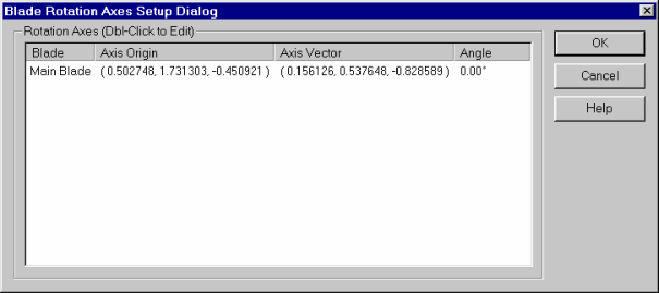
The Blade Rotation Axis Specification Dialog (second dialog below) provides access to a blade’s rotation settings. It is displayed initially if only one blade exists, or when the user double-clicks on a blade’s description in the Blade Rotation Axes Setup Dialog. Using this dialog, the user may specify the Meridional Fraction, Pitch Fraction and Axis Angle for the new rotation axis as well as the Rotation Angle for the blade (right-hand rule).
Note: The origin of the rotation axis will always lie on the hub. The axis angle applies to the meridional view, with a zero degree line being positive and to the right.
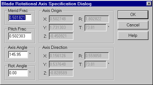
Once the rotation parameters have been set up, the rotation axis will be available for display in both the Meridional View and 3D View. The final step is to apply the blade rotation by selecting the Tools | Rotate Blades about Axes menu command.