In order to model a free surface using the VOF model, perform the following steps in Ansys Polydata:
Create a VOF task by clicking Create a new task.
 Create a new task
Then perform the following actions in the Create a new task menu:
Specify that the VOF model is used for this task by clicking Volume Of Fluid problem(s).
Volume Of Fluid problem(s)
Set up the geometry type.
Click Accept the current setup to open the VOF task menu.
Create the flow sub-task in the usual manner.
Create a sub-task
Note the following:
Some of the menu items in the Flow boundary condition along boundary <ID> are not available for VOF tasks.
As a VOF simulation is transient, it is recommended that you use a nonvanishing density and take inertia terms into account (especially for viscoelastic fluids, for which inertia has a stabilizing effect). These settings can be made using the Material Data menu.
After the flow sub-task is defined, a fluid fraction transport sub-task named F.E.M. Task Fluid Fraction Transport is automatically created and listed in the task menu. Click this menu item to begin defining the sub-task.
F.E.M. Task Fluid Fraction Transport
The F.E.M. Task Fluid Fraction Transport menu will open.
Click Domain of the sub-task and define the domain of the fluid fraction transport sub-task in the usual way. Note that this domain represents the cavity in which the fluid will be tracked.
Domain of the sub-task
Define where the initial fluid is present (that is, the fluid already in the cavity when the simulation starts) by clicking Material data.
Material data
The Material Data menu will open, where you can perform the following steps.
To define the initial fluid fraction distribution, click Initial Fluid Fraction. When tracking a single fluid, the fluid is determined to be present wherever the fluid fraction is between 0.5 and 1; while this range of values is acceptable, it is recommended that you set the fluid regions to a value of 1 if possible. Similarly, the fluid is determined to be absent wherever the fluid fraction is lower than 0.5, but it is recommended that the empty regions have a value of 0. By default, the initial fluid fraction is set to 0 throughout the domain.
Initial Fluid Fraction
The Initial Fluid Fraction menu will open, allowing you to define the initial fluid fraction as being:
a constant value
You can specify that the value of the fluid fraction is the same throughout the domain by clicking Constant.
Constant
A panel will open where you can enter the fluid fraction for New value. Click OK to return to the Initial Fluid Fraction menu.
a linear function
You can specify that the fluid fraction is defined as a linear function of the coordinates (
 ), as shown in the following equation:
(21–3)
Click Linear function of coordinates.
Linear function of coordinates
Panels will open where you can revise the New value for the parameters A, B, C, and D of the previous equation. Click in the final panel to return to the Initial Fluid Fraction menu.
a multi-ramp function
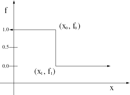
You can specify the fluid fraction behaves as a multi-ramp function that is defined by a sequence of coordinate pairs. For example, if you choose to vary the fluid fraction
 as a function of the
  coordinates, you will input pairs of
coordinates
coordinates, you will input pairs of
coordinates  (where
  begins at 0 and is incremented for each
additional pair). See Figure 21.3: A Multi-Ramp Function for the Initial Fluid
Fraction for an illustration of a multi-ramp
function.
begins at 0 and is incremented for each
additional pair). See Figure 21.3: A Multi-Ramp Function for the Initial Fluid
Fraction for an illustration of a multi-ramp
function. Click the appropriate multi-ramp menu item based on the axis for which the values will vary.
Multi-ramp function of X coordinate
or
Multi-ramp function of Y coordinate
or
Multi-ramp function of Z coordinate
The ffinit = Multi-ramp function on <direction> coordinate menu will open, where you can perform the following:
To input the coordinate pairs, select Define new pairs and enter the coordinate values in the panels that open.
To review the coordinate pairs you defined, click Check existing pairs. You can delete a pair by clicking Delete mode and then clicking the pair. You can modify the values by clicking Modify mode, clicking the pair, and then entering values in the panels that open. When you have determined that the pairs are all correctly defined, click Upper level menu to return to the previous menu.
To save the coordinate pair data for future use, click Save in a Dependence Data File and use the panel that opens to create a data file. This file can be recalled later by using the Read in a Dependence Data File menu item, as explained in the description that follows.
To input the coordinate pairs using a previously written data file instead of interactively entering the pairs, click Read a Dependence Data File and select the file using the panel that opens. You could have created such a data file using the Save in a Dependence Data File menu item as described previously, or using another tool that writes the pairs of data in the fixed (Fortran) format 2e14.7. Each data pair (e.g.,
 ,
,  ) is written on a single line, and
fourteen digits are used for representing each datum as
) is written on a single line, and
fourteen digits are used for representing each datum as
 0.1234567e
 89. Because the format is fixed, there
is no need to use a separator. The following is a list
(in order) of the components of a single datum in the
e14.7 format: a sign, a 0 digit, the decimal point,
seven digits (for the mantissa), the letter "e"
(standing for a power of 10), a sign for the power, and
two digits (for the power). For example, an entry in the
file that represents (0.25,-
89. Because the format is fixed, there
is no need to use a separator. The following is a list
(in order) of the components of a single datum in the
e14.7 format: a sign, a 0 digit, the decimal point,
seven digits (for the mantissa), the letter "e"
(standing for a power of 10), a sign for the power, and
two digits (for the power). For example, an entry in the
file that represents (0.25,-  ) would be written as
+0.2500000e+00-0.31415926e+01. Subsequent data pairs are
written on subsequent lines.
) would be written as
+0.2500000e+00-0.31415926e+01. Subsequent data pairs are
written on subsequent lines.
Click Upper level menu when finished defining the multi-ramp function to return to the Initial Fluid Fraction menu.
interpolated values from a CSV (Excel) file
You can interpolate fluid fraction values onto your mesh from a comma separated values (CSV) file, in a way similar to that described in Results Interpolation Onto Another Mesh. The CSV file could have been created using a mesh that has different nodal locations, but the same overall geometry. Click Map from CSV (Excel) file.
Map from CSV (Excel) file
The Map from CSV file menu will open. Click Modify the CSV file name and use the panel that opens to select the file. Then click Modify the label, enter a case sensitive tag for New value in the panel that opens to identify the data, and click . Finally, click Upper level menu to return to the Initial Fluid Fraction menu
a user-defined function (UDF)
You can specify that the fluid fraction is defined using a UDF by clicking User-defined function.
User-defined function
See User-Defined Functions (UDFs) for information about UDFs.
Click Upper level menu to return to the Material Data menu.
To save the initial fluid fraction data defined using the Initial Fluid Fraction menu item for future use, click Save in a Material Data File.
Save in a Material Data File
A panel will open, which you can use to create a material data file. This file can be recalled later by using the Read an Old Material Data File menu item, as explained in the description that follows.
To input the initial fluid fraction using a previously written material data file (instead of inputting it using the Initial Fluid Fraction menu item), click Read an Old Material Data File. You could have created such a material data file using the Save in a Material Data File menu item, as described previously.
Read an Old Material Data File
A panel will open, which you can use to select the material data file.
Click Upper level menu to return to the F.E.M. Task Fluid Fraction Transport menu.
Define the boundary conditions for the fluid fraction transport sub-task.
Fluid Fraction boundary conditions
The Fluid Fraction boundary conditions menu will open, where you can perform the following:
Select a boundary for which you want to define the boundary condition.
Click Modify to open the Fluid Fraction boundary condition along boundary <ID> menu.
Select the boundary condition type you want to impose:
Click Inlet if you want to specify that the boundary allows the fluid you are tracking to enter the domain. Note that all boundaries specified as an Inlet are taken into account when the mass balance is computed.
Inlet
Enter the fluid fraction for New value in the panel that opens and click OK. When tracking a single fluid, the New value must be set to
1for an inlet.Then click Upper level menu to return to the previous menu.
Note that it is possible to make your Inlet boundary condition variable with time by using the button (as described in Problem Setup), in order to simulate variable injection. You must make sure that at every time step the fluid fraction for the inlet is either 0 or 1.
Click Fluid Fraction imposed if you want to force a boundary to be either wet or dry, and thereby fine-tune a simulation to better match expected behavior. Note that all boundaries specified as a Fluid Fraction imposed are not taken into account when the mass balance is computed.
Fluid Fraction imposed
Enter the fluid fraction for New value in the panel that opens and click . When tracking a single fluid, the New value should be set to
1for a wet boundary and0for a dry boundary.Then click Upper level menu to return to the previous menu.
Click Wall / Symmetry if you want to specify that the boundary acts as a wall for the fluid you are tracking, such that no fluid enters or exits (which is the equivalent of a symmetry boundary).
Wall / Symmetry
Click Outlet if you want to specify that the boundary allows the fluid you are tracking to exit the domain. Note that all boundaries specified as an Outlet are taken into account when the mass balance is computed.
Outlet
Click Source of connected condition to specify that the boundary acts as a "source" boundary in a pair of non-conformal boundaries that are to be connected. It is recommended that the source be the coarser of the two meshes. Non-conformal boundary conditions are described in Non-Conformal Boundaries.
Source of connected condition
Click Target of connected condition to specify that the boundary acts as a "target" boundary in a pair of non-conformal boundaries that are to be connected. This menu item is only available if you have defined a source boundary, as described previously. It is recommended that the target be the finer of the two meshes. Non-conformal boundary conditions are described in Non-Conformal Boundaries.
Target of connected condition
The Target of connected cond. along boundary <ID> menu will open, where you must select a boundary from the list and click Select. Then the Options for connected boundaries menu will open, where you can set the parameters for the non-conformal boundary.
The inputs for non-conformal fluid fraction boundary conditions are the same as those for flow boundary conditions, as described in Connecting Non-Conformal Boundaries, except for the numerical parameters. The first two numerical parameters (element dilatation and amplitude of volume generation) are the same as for flow boundary conditions, but the stabilization factor for flow conditions is replaced by a smoothing factor for fluid fraction conditions. The smoothing factor controls the fluid fraction transport tangential to the surface of the connected boundaries. Ideally, there should be no fluid fraction transport within the connected boundaries, but setting this parameter to zero can lead to numerical problems (for example, zero pivot) or instabilities. It is therefore recommended to set the smoothing factor to a very small nonzero value.
Important: Changing the value of the smoothing factor from the default value is not recommended, except on the advice of your support engineer.
Click Upper level menu to return to the Fluid Fraction boundary conditions menu.
Repeat steps 6.(a)–6.(c) for each additional boundary you want to define.
Click Upper level menu to return to the F.E.M. Task Fluid Fraction Transport menu.
Click Upper level menu to return to the VOF task page.
Modify the numerical parameters for the VOF task.
Numerical parameters
The Numerical parameters menu will open.
Define the iterative parameters for the VOF task, by clicking Modify the VOF iterative parameters.
Modify the VOF iterative parameters
The VOF iterative parameters menu will open.
Specify the time at which the time-marching procedure begins.
Modify the initial time value
Enter the initial time for New value in the panel that opens and click .
Specify the time by which the solution procedure must stop.
Modify the upper time limit
Enter the latest permissible end time for New value in the panel that opens and click OK.
Define the value of
 for the initial time step.
Modify the initial value of the time-step
for the initial time step.
Modify the initial value of the time-step
Enter the initial
 for New value in the
panel that opens and click . Note that
the elapsed time for a time step is set to this value when the
inlet flow rate is 0, so it is recommended that you enter a
conservative value.
for New value in the
panel that opens and click . Note that
the elapsed time for a time step is set to this value when the
inlet flow rate is 0, so it is recommended that you enter a
conservative value. Define the minimum allowable value of
 for any time step.
Modify the min value of the time-step
for any time step.
Modify the min value of the time-step
Enter the minimum
 for New value in the
panel that opens and click .
for New value in the
panel that opens and click . Define the maximum allowable value of
 for any time step.
Modify the max value of the time-step
for any time step.
Modify the max value of the time-step
Enter the maximum
 for New value in the
panel that opens and click .
for New value in the
panel that opens and click . Define the accuracy of the VOF scheme (
 in Equation 21–2).
Modify the accuracy of the VOF scheme
in Equation 21–2).
Modify the accuracy of the VOF scheme
Enter the accuracy for New value in the panel that opens and click OK. It is recommended that the accuracy be on the order of 0.2–0.5.
Define the maximum number of successful (that is, converged) steps. The computation will be stopped when this number is reached, even if the upper time limit has not yet been reached. Note that you can always restart the scheme from the results file in order to continue the time-marching scheme without losing the benefit of the previous solutions. See Starting an Ansys Polyflow Calculation from an Existing Results File for more information on these file types.
Modify the max number of successful steps
Enter the maximum number of steps for New value in the panel that opens and click .
If you would like the simulation to run when the flow balance is zero (that is, the total outlet flow rate is over 99% of the nonzero total inlet flow rate) or when the entire domain exceeds the fluid fraction threshold (that is, the cavity is filled with fluid), you can disable the default constraint that limits this behavior by clicking the Disable ‘Stop When Full’ criterion menu item.
Disable ‘Stop When Full’
criterion
This menu option then becomes Enable ‘Stop When Full’ criterion, so that you can toggle it back if necessary.
Select the method of integration by clicking one of the following:
-
Use of the O-order method
-
Use of the implicit Euler method
-
Use of the Galerkin method
-
Use of the Crank-Nicolson method
See Integration Methods for details about the previous integration methods.
Click Upper level menu to return to the Numerical parameters menu.
Click Upper level menu to return to the VOF task menu.