


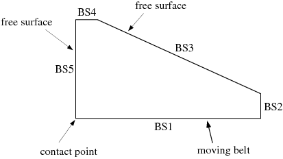
A contact problem occurs at points (in 2D) or lines (in 3D) where the velocity is fixed and the position of the free surface or moving interface is not prescribed. In this case, you have a moving contact point (or line). Consider, for example, the curtain coater shown in Figure 15.12: Example of a Contact Point. The flow enters at a constant speed at the top of the domain (BS4) and falls onto a belt that moves horizontally (BS1). The problem involves two free surfaces: one on the right (BS3) and one on the left (BS5). The fluid is carried by the belt, and the point located at the intersection between the belt and the left free surface is a contact point. The position of free surface BS5 is not known, and the velocity is imposed based on the motion of the belt.
Since the position of the moving surface at the contact point is not prescribed, a contact angle is prescribed between the free surface and the adjacent boundary.
If your problem includes a point or line where the velocity is fixed and the position of the free surface or moving interface is not prescribed, Ansys Polydata will automatically request input of the contact angle, and implement the moving-contact-point strategy.
Ansys Polydata will warn you if the model is incoherent (that is, if a velocity has not been imposed at a location where the free-surface or moving-interface position has been imposed, or in a moving-contact-point problem if the director has not been imposed).
Contact points are, in some sense, a paradox, since the Lagrangian kinematic
requirement  readily describes the displacement on such points. If
 , these points or lines do not move. In the numerical
simulation, however, you may want to include additional effects such as
capillary forces, which bring the fluid back to the wall when sharp free-surface
or moving-interface gradients exist.
, these points or lines do not move. In the numerical
simulation, however, you may want to include additional effects such as
capillary forces, which bring the fluid back to the wall when sharp free-surface
or moving-interface gradients exist.
The moving-contact-point model allows you to take these additional effects
into account. This model can be used whenever the capillary number
 is not too large. The capillary number
  measures the importance of viscous forces compared to
capillary forces:
measures the importance of viscous forces compared to
capillary forces:
 | (15–23) |
where  is the viscosity and
  is a characteristic velocity of the flow.
For contact problems that do not include surface tension (or when the capillary number is large), the time-dependent approach of Blow Molding and Thermoforming must be used instead of the moving-contact-point model.
When surface tension is present, you will need to specify a static contact
angle wherever the moving-boundary position is not prescribed. This angle is
called static because it will be respected only in the limit of small viscous
forces (that is, when capillary forces dominate all other forces). This angle
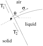
corresponds to the wetting angle ( in Equation 15–20) between the fluid and the wall, as shown in Figure 15.13: Static Contact Angle.
The wetting angle is completely determined by the interfacial force balance at a triple point in situations where the fluid does not move and therefore does not generate viscous or inertial forces. If the fluid moves, viscous (and possibly inertial) forces will be combined with the surface tension force (which is tangent to the free surface, as described in Surface Tension), and the point will move up to a position where the projection of the resulting force on the direction tangent to the wall vanishes.
This assumes that the moving contact point has no mass in itself, and that momentum equilibrium is satisfied in the direction tangent to the wall. In a direction normal to the wall, no displacement is allowed.
To use the moving-contact-point model in Ansys Polyflow, follow the guidelines below when setting up your model in Ansys Polydata:
Be sure that your model actually involves a moving contact point (that is, a velocity boundary condition is prescribed on the boundary adjacent to the free surface, surface tension is included, and a wetting angle is prescribed). As discussed in Surface Tension, positive angles are measured counterclockwise with respect to a horizontal reference axis (see Figure 15.3: Surface Tension and Traction at the Extremities of a Free Surface).
Prescribe the director of the contact point as the tangent direction to the wall. This means that moving-contact-point problems can be modeled only for straight lines, since only a constant director can be specified.
In practice, moving-contact-point problems can be steady-state as well as time-dependent. For the steady-state case, the kinematic condition degenerates into a dynamic condition that states the equilibrium of the tangential forces. However, in most moving-contact-point problems, it is likely that a time-dependent approach will be more computationally stable than a steady-state approach. A time-dependent approach guarantees that the displacements will be small, provided that the time steps are small. Using a transient scheme is therefore highly recommended.
If the surface tension is very small, the only way to handle a moving contact point is by using a time-dependent scheme with contact detection (penetration check). See Blow Molding and Thermoforming for details.
Ansys Polydata will replace the kinematic condition (Equation 15–2 or Equation 15–3) by the momentum balance in the direction tangent to the wall. Therefore, the static angle will be taken into account in the momentum balance, although the Dirichlet boundary condition prescribed on the velocity field supersedes this momentum equation.
If the free surface is normal to the wall, perfect wetting occurs. In this case, the direction tangent to the wall is also normal to the free surface, so the director never becomes tangent to the free surface. Conversely, if the free surface becomes tangent to the wall, no wetting occurs and the direction tangent to the wall is also tangent to the free surface. This results in an ill-posed problem, as discussed in Free Surfaces. In this case, the only option is to use a contact detection algorithm such as that described in Blow Molding and Thermoforming.